Partially Observable MDPs (POMDPs)

A POMDP is an MDP where you cannot see the true state, so you plan from a belief: a probability distribution over where you might be. Every observation reshapes that belief with Bayes' rule, and the policy maps beliefs to actions.

Two left growls move the belief that the tiger is behind the left door from 0.50 to 0.85 to 0.97.

Why Does This Exist?

Markov decision processes assume the agent always sees the true state. Most interesting problems refuse that deal. In poker you never see the hole cards. A delivery robot gets noisy sonar pings, not a map coordinate. A doctor sees symptoms and test results, never the disease itself. In each case the same observation can demand different actions depending on a hidden truth, so a policy that maps observations straight to actions is playing blindfolded with one eye open.

The fix is to stop pretending the observation is the state. Instead the agent keeps a belief: a probability distribution over the hidden states, updated every step as actions are taken and observations arrive. Decisions then come from the belief, which squeezes every drop of evidence out of a history the agent could never store raw.

This page covers the POMDP tuple, the exact belief update with worked numbers, and why planning over beliefs is fundamentally hard. It assumes you know the MDP setup; if states, actions and discounted return are new, read the MDP page first. A follow-up page on belief states will go deeper into how beliefs are represented and approximated in large problems.

Think of It Like This

The Dark Apartment and the Flickering Flashlight

You come home to a blackout and your keys could be in the kitchen, on the couch, or in the hallway. You cannot see them, so you carry odds in your head: say 50% kitchen, 30% couch, 20% hallway. That running set of odds is your belief.

Your flashlight is dying, so each flicker gives you one unreliable glimpse. A glint from the kitchen direction does not mean the keys are there. It just shifts the odds: kitchen up, the rest down. And you pick the next room to search from the odds, not from a sighting you never had. Two glints from the kitchen in a row and you walk straight there. A glint from the hallway right after cancels the first one out and you are back to square one.

Where the analogy stops: your searching never moves the keys. In a POMDP, actions usually change the hidden state too, so the belief has to predict motion as well as weigh evidence. The tiger example below uses listening actions that leave the tiger put, which keeps the arithmetic clean.

How It Actually Works

A POMDP is the tuple $(S, A, T, R, \Omega, O, \gamma)$ . $S$ is a finite set of hidden states, the truths the agent never sees directly. $A$ is the finite action set. $T(s' \mid s, a)$ is the transition model, the probability of landing in state $s'$ after taking action $a$ in state $s$ . $R(s, a)$ is the expected immediate reward. $\Omega$ is the finite observation set, the sensor readings the agent actually receives. $O(o \mid s', a)$ is the observation model, the probability of seeing $o$ after arriving in $s'$ via $a$ . $\gamma$ in $[0, 1)$ discounts future reward exactly as in an MDP.

Because the state is hidden, the agent conditions on the full history of actions and observations. The belief $b(s)$ compresses that history into one object: the probability the current state is $s$ , with $b(s) \ge 0$ and $\sum_s b(s) = 1$ . The policy then maps beliefs to actions, $\pi(b)$ , instead of states to actions.

The belief update

Taking action $a$ and seeing observation $o$ turns the old belief $b$ into a new belief $b'$ through Bayes' rule:

$b'(s') = \eta \, O(o \mid s', a) \sum_{s \in S} T(s' \mid s, a) \, b(s)$

Read it right to left. The sum predicts where you might be now: each old possibility $b(s)$ flows through the transition model. The observation model then weighs each candidate by how well it explains what you just saw. $\eta$ is the normalizer, one over the total probability of that observation, which forces the new belief to sum to 1. Nothing here is learned or tuned. Given the models and the evidence, this is the only consistent new belief.

Beliefs turn the POMDP back into a fully observable problem called the belief MDP. Its "states" are beliefs, which form a continuous simplex rather than a finite set. Its reward in belief $b$ is the expected immediate reward $\sum_s b(s) R(s, a)$ , and its transitions come from the update above plus the chance of each observation. The optimal value function over this belief space has a special shape: it is piecewise linear and convex, representable as the upper surface of a set of hyperplanes called alpha vectors. Each backup adds hyperplanes the same way value iteration adds Bellman backups, except the backup ranges over a continuum of beliefs.

Worked example: the two-state tiger

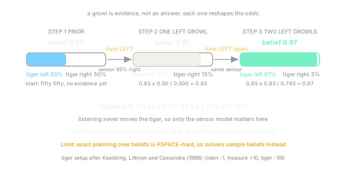
The tiger problem from Kaelbling, Littman and Cassandra (1998) has two hidden states: the tiger is behind the left door ( $TL$ ) or the right door ( $TR$ ). Three actions: listen (cost $-1$ , tiger stays put), open left, open right (treasure $+10$ behind the tiger-free door, tiger $-100$ behind the other). Listening reports the tiger's side correctly 85% of the time, so $O(\text{left} \mid TL, \text{listen}) = 0.85$ and $O(\text{left} \mid TR, \text{listen}) = 0.15$ . Because listening never moves the tiger, the transition sum drops out and the update is pure weighing plus normalization.

Start fifty fifty: $b(TL) = 0.50$ . You listen and hear a growl from the left.

Numerators: $0.85 \times 0.50 = 0.425$ for $TL$ , $0.15 \times 0.50 = 0.075$ for $TR$ . Normalizer: $0.425 + 0.075 = 0.500$ . Posterior: $b'(TL) = 0.425 / 0.500 = 0.85$ . One growl moves fifty fifty to 0.85.

Listen again, hear left again. Numerators: $0.85 \times 0.85 = 0.7225$ for $TL$ , $0.15 \times 0.15 = 0.0225$ for $TR$ . Normalizer: $0.7225 + 0.0225 = 0.745$ . Posterior: $b''(TL) = 0.7225 / 0.745 = 0.9698$ , about 0.97. The second matching growl nearly settles it.

Conflicting evidence cancels. From 0.85, a growl from the right gives numerators $0.15 \times 0.85 = 0.1275$ and $0.85 \times 0.15 = 0.1275$ , normalizer $0.255$ , posterior $0.1275 / 0.255 = 0.50$ . Right back where you started.

Beliefs then drive the decision through expected value. At $b(TL) = 0.85$ , opening the right door nets $0.85 \times 10 - 0.15 \times 100 = -6.5$ , worse than paying $-1$ to listen again. At $b(TL) = 0.97$ , opening the right door nets $0.97 \times 10 - 0.03 \times 100 = +6.7$ , so the agent stops listening and opens. That threshold behavior, keep sensing while unsure and commit once the belief is sharp, is the signature POMDP policy shape.

Why exact solving is hard

The belief space is continuous, so the alpha-vector set behind the exact value function can grow without bound. Finding an optimal finite-horizon policy is PSPACE-hard (Papadimitriou and Tsitsiklis, 1987), and exact infinite-horizon planning is undecidable. That is why practical solvers never plan over all beliefs. Point-based methods such as PBVI and SARSOP keep alpha vectors only at a sampled set of beliefs the agent is actually likely to visit, and trade optimality for a bound on how much value the sampling loses.

Code

A standalone Python check of the tiger belief updates above. Every printed number is the update formula evaluated, not typed in.

1def belief_update(prior_left: float, heard_left: bool, accuracy: float = 0.85) -> float:2    """One Bayes update for the two-state tiger problem."""3    hit = accuracy if heard_left else 1.0 - accuracy4    miss = 1.0 - accuracy if heard_left else accuracy5    num = hit * prior_left6    return num / (num + miss * (1.0 - prior_left))7
8
9b0 = 0.5010b1 = belief_update(b0, heard_left=True)11b2 = belief_update(b1, heard_left=True)12b3 = belief_update(b1, heard_left=False)13print(f"prior {b0:.2f} -> hear left: {b1:.2f}")14print(f"prior {b1:.2f} -> hear left: {b2:.4f}")15print(f"prior {b1:.2f} -> hear right: {b3:.2f}")

1# -> expected output:2prior 0.50 -> hear left: 0.853prior 0.85 -> hear left: 0.96984prior 0.85 -> hear right: 0.50

Watch Out For

Feeding raw observations into an MDP policy

The classic shortcut is to treat each observation as if it were the state and run standard temporal-difference learning on it. That breaks under perceptual aliasing: two different hidden states emit the same observation, so one observation needs two different actions and a single policy entry cannot hold both. The symptom looks like a tuning problem. The agent dithers between moves at the aliased observation, or learns the average action, which is wrong everywhere.

Fix it by deciding from the belief or the history, never from one observation. Keep the Bayes update running, or use a recurrent policy that carries history, and watch the aliased cases separate once the policy sees what the single snapshot hides.

Acting on the most likely state instead of the belief

Once the belief leans left at 0.85, the temptation is to declare the tiger found and open the right door. The most likely state is not a decision. Opening at 0.85 nets $-6.5$ in expectation because the 15% chance of a $-100$ mistake dominates the $+10$ prize. The symptom is an agent that senses just enough to feel confident and then eats catastrophes at exactly the rate its sensor lies.

Fix it by comparing expected values over the full belief, as the worked example does: listen while opening loses money, commit only when the belief is sharp enough that the math flips. Uncertainty is an input to the decision, not noise around it.

The Quick Version

A POMDP adds hidden state to the MDP: the agent receives observations, never states, so the policy must act from a belief distribution over where it might be.
The belief update is Bayes' rule. Predict forward through the transition model, weigh each candidate by how well it explains the observation, then normalize.
Two 85%-accurate left growls move P(tiger left) from 0.50 to 0.85 to 0.97, while one conflicting growl drops it back to 0.50.
Decisions compare expected values over the belief. At 0.85, opening nets $-6.5$ so the agent keeps listening. At 0.97, opening nets $+6.7$ so it commits.
Exact finite-horizon planning is PSPACE-hard, so practical solvers plan over a sampled set of likely beliefs instead of the whole belief space.