Value Iteration
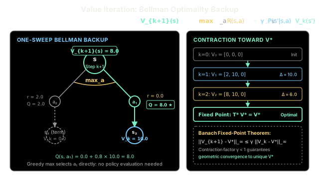
Value iteration converges directly to the optimal state values by updating each state with the best possible immediate action and next-state return in a single Bellman backup.
Why Does This Exist?
In reinforcement learning, when an agent possesses complete knowledge of the environment's transition dynamics and reward model—formalized as a Markov Decision Process—it can compute the optimal policy directly using dynamic programming.
The classic approach, Policy Iteration, decomposes this goal into two strict, alternating phases:
- Policy Evaluation: Compute the exact state values for the current policy , which requires either inverting a transition matrix or running many iterative sweeps until values converge to high precision.
- Policy Improvement: Greedily update the policy with respect to the freshly calculated .
In practice, full policy evaluation is computationally wasteful. The greedy action choices often lock into their optimal choices after only a few sweeps, long before the numerical value estimates converge to multiple decimal places.
Value Iteration solves this inefficiency by truncating policy evaluation after exactly one sweep. Instead of evaluating a candidate policy to convergence before improving it, Value Iteration merges evaluation and greedy improvement into a single update. Every sweep directly applies the Bellman optimality equation with a operator over all possible actions. The algorithm operates entirely in value space, deferring explicit policy extraction until the value function has contracted to near-optimality.
Think of It Like This
Filling a lake with water: propagation to equilibrium
Imagine a tiered network of mountain reservoirs and dry riverbeds down-slope from a glacial waterfall (the primary reward source).
At the start (), every dry basin across the landscape has an estimated water level of zero ().
On the first day, the waterfall pours directly into the top tier of reservoirs immediately adjacent to it, raising their water level to reflect the immediate influx. On the second day, those newly elevated reservoirs spill outward into the next tier of reservoirs downstream. Water levels propagate outward, one elevation step per cycle, driven by hydraulic gradients.
Each basin updates its water height based strictly on the highest inflow sluice gate connected to it (the over actions), discounted by the frictional resistance of distance (the discount factor ).
Crucially, hydraulic engineers do not need to pause and simulate microscopic eddy currents until perfect molecular stillness (full policy evaluation) before allowing water to spill forward. Each discrete surge propagates the highest incoming level to the next pool. Cycle after cycle, the flood front advances across the entire mountain until water levels everywhere stabilize in hydrostatic equilibrium ().
Where the analogy stops: Physical fluids conserve mass, obey momentum, and follow continuous Navier-Stokes equations. Value Iteration operates through discrete mathematical projections over state spaces, where future returns are geometrically discounted by rather than governed by physical mass conservation.
How It Actually Works
The Bellman optimality operator and truncated policy evaluation
Consider a finite Markov Decision Process , where:
- is the finite set of environmental states.
- is the set of actions available in state .
- is the joint transition and reward probability function.
- is the temporal discount factor.
The optimal state-value function represents the maximum expected discounted return attainable from state under any policy. It satisfies the non-linear Bellman Optimality Equation:
Equivalently, letting expected immediate reward be and transition dynamics be :
Value Iteration turns this mathematical identity into an iterative update rule. Starting with an arbitrary initial value array (typically all zeros), it repeatedly updates each state:
The Bellman optimality operator ()
We can define the Bellman optimality backup as an operator :
Value iteration is simply the successive application of this operator: .
Contraction mapping and convergence guarantee
Under the supremum norm (infinity norm) , the operator is a -contraction mapping:
Because , the Banach Fixed-Point Theorem delivers three vital guarantees:
- Uniqueness: There is exactly one fixed-point value function such that .
- Global convergence: Starting from any arbitrary initial vector , the sequence converges to as .
- Geometric rate: The distance to the optimal value function shrinks by at least factor on every sweep:
Stopping threshold and policy extraction
In practice, sweeps continue until the maximum change across all states falls below a small positive tolerance :
Once convergence is reached, the deterministic optimal policy is extracted through a single one-step greedy lookahead:
Worked numerical example
Consider an MDP with 3 states and discount factor .
- State is a terminal absorption state: .
- Actions available in non-terminal states are :
- From :
- Action advances to with : .
- Action exits immediately to terminal with : .
- From :
- Action exits directly to terminal with high reward : .
- Action loops back to with minor reward : .
- From :
Initialization ()
Sweep 1 ()
Calculate candidate action values for each state:
- For :
- For :
Max change: .
Sweep 2 ()
Apply the Bellman optimality backup using updated values :
- For :
- For :
Max change: .
The high downstream reward at has backed up into . The greedy choice at flipped from the immediate short-term reward of () to the delayed path ().
Sweep 3 ()
- For : .
- For : .
Max change: .
The values have converged exactly in 3 sweeps:
- Optimal values: .
- Optimal policy: .
Code
from typing import Dict, List, Tuple
def value_iteration( states: List[int], actions: List[int], transitions: Dict[Tuple[int, int], List[Tuple[float, int, float]]], gamma: float = 0.8, theta: float = 1e-6,) -> Tuple[Dict[int, float], Dict[int, int]]: """ Computes the optimal value function and policy using Value Iteration.
Args: states: List of state identifiers. actions: List of action identifiers. transitions: Mapping of (s, a) -> list of (probability, s_next, reward). gamma: Discount factor in range [0, 1). theta: Convergence threshold for stopping sweeps.
Returns: V: Optimal state values mapping state to value. policy: Optimal deterministic policy mapping state to best action. """ V: Dict[int, float] = {s: 0.0 for s in states}
while True: delta: float = 0.0 V_new = V.copy()
for s in states: q_values: Dict[int, float] = {} for a in actions: outcomes = transitions.get((s, a), []) if outcomes: q_values[a] = sum( prob * (reward + gamma * V[s_next]) for prob, s_next, reward in outcomes )
if q_values: best_value = max(q_values.values()) delta = max(delta, abs(best_value - V[s])) V_new[s] = best_value
V = V_new if delta < theta: break
# Extract optimal policy via 1-step greedy lookahead policy: Dict[int, int] = {} for s in states: q_values = {} for a in actions: outcomes = transitions.get((s, a), []) if outcomes: q_values[a] = sum( prob * (reward + gamma * V[s_next]) for prob, s_next, reward in outcomes ) if q_values: policy[s] = max(q_values, key=lambda a: q_values[a])
return V, policy
# Environment configuration: 3-state MDP matching worked example# States: 0 (s1), 1 (s2), 2 (s3 terminal)# Actions: 0 (a1), 1 (a2)transitions: Dict[Tuple[int, int], List[Tuple[float, int, float]]] = { (0, 0): [(1.0, 1, 0.0)], # (s1, a1) -> s2, r=0.0 (0, 1): [(1.0, 2, 2.0)], # (s1, a2) -> s3, r=2.0 (1, 0): [(1.0, 2, 10.0)], # (s2, a1) -> s3, r=10.0 (1, 1): [(1.0, 0, 1.0)], # (s2, a2) -> s1, r=1.0}
states = [0, 1, 2]actions = [0, 1]
optimal_values, optimal_policy = value_iteration( states=states, actions=actions, transitions=transitions, gamma=0.8, theta=1e-6,)
print("Optimal Values:", {f"s{s+1}": round(v, 2) for s, v in optimal_values.items()})print("Optimal Policy:", {f"s{s+1}": f"a{a+1}" for s, a in optimal_policy.items()})# -> Optimal Values: {'s1': 8.0, 's2': 10.0, 's3': 0.0}# -> Optimal Policy: {'s1': 'a1', 's2': 'a1'}Watch Out For
Stopping before value differences are small enough
A common failure mode is assuming that when successive sweep differences fall below (), the current values are within of the true optimal values .
Because errors accumulate across future horizons through the discount factor , the true distance to optimality satisfies:
More dangerously, the policy derived greedily from has an amplified suboptimality bound:
When , the multiplier . Stopping with a loose threshold like can yield an extracted policy that is up to units of return worse than the true optimal policy.
The Fix: When requiring a policy within target suboptimality tolerance , calibrate your stopping threshold to:
The Quick Version
- Value Iteration truncates policy evaluation after a single sweep, directly combining evaluation and greedy improvement into a single Bellman optimality backup.
- It operates strictly in value space without maintaining or evaluating intermediate policies; an optimal policy is extracted via greedy lookahead once values converge.
- The Bellman optimality operator is a -contraction mapping under the infinity norm, guaranteeing geometric convergence to a unique optimal value function .
- Calibrate the stopping threshold against to prevent terminating prematurely when is close to 1.