Phasic Policy Gradient (PPG)

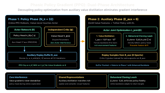
Phasic Policy Gradient decouples feature representation learning from policy optimization by alternating between an online policy phase and an offline auxiliary phase with policy cloning.

Phasic Policy Gradient alternates between an online policy phase and an auxiliary distillation phase with behavioral cloning to prevent policy drift.

Why Does This Exist?

In deep reinforcement learning, Actor-Critic algorithms face a fundamental architectural dilemma regarding shared representation learning:

The Argument for Sharing: Training neural networks on raw sensory inputs (such as Atari pixels or robotic camera streams) requires discovering rich spatial and temporal features. Value prediction is a dense, high-signal regression task: every single state provides a scalar Bellman return target $\hat{V}$ . Sharing early convolutional and trunk layers between the policy head $\pi(a \mid s)$ and value head $V(s)$ forces the network to learn robust visual representations much faster than learning from sparse policy gradient rewards alone.
The Destructive Interference Problem: Value function regression targets exhibit large gradient magnitudes and high variance. When the value head and policy head backpropagate through shared trunk weights simultaneously, value function updates violently distort the latent features. These sudden representation shifts destabilize the policy head $\pi(a \mid s)$ , causing performance degradation and premature policy entropy collapse.
The Disjoint Network Compromise: If an engineer completely decouples the networks—using one isolated neural network for the Actor and a separate network for the Critic—gradient interference is eliminated. However, the Actor no longer benefits from the rich visual representations discovered by the Critic, requiring orders of magnitude more environment interactions to achieve competence.

Introduced by Cobbe et al. (OpenAI, 2021), Phasic Policy Gradient (PPG) resolves this dilemma. PPG decouples policy optimization from representation learning across two distinct alternating phases. By restricting online policy updates to pure policy gradients and relegating value representation distillation to a periodic offline auxiliary phase protected by a behavioral policy cloning constraint, PPG achieves the representation-sharing sample efficiency of joint networks with the optimization stability of disjoint networks.

Think of It Like This

Field Expeditions vs. Laboratory Analysis

Imagine an environmental biologist conducting research on a dangerous, unpredictable wilderness reserve:

The Standard Approach (Running Assays While Fleeing Predators): Imagine trying to calibrate an ultra-sensitive mass spectrometer while simultaneously sprinting through thick brush to evade wild predators. Attempting to balance delicate biochemical analysis (value regression) with survival reflexes (policy gradient) guarantees failure: you will either drop the spectrometer or get caught by the predator.
The PPG Approach (Alternating Phasic Cycles):
- The Policy Phase (Field Expedition): You step out into the field with one sole objective: navigation and survival. Your physical reflexes ( $\pi_{\boldsymbol{\theta}}$ ) are dedicated entirely to exploring, dodging hazards, and collecting interesting soil and water samples. You do not run any complex chemical assays in the field; you simply store the samples and your GPS trajectory into a backpack (the auxiliary replay buffer $\mathcal{B}_{\text{aux}}$ ).
- The Auxiliary Phase (The Base Camp Laboratory): Every few weeks, you return to a sterile base camp laboratory. Over multiple quiet rounds of analysis ( $E_{\text{aux}}$ epochs), you test your accumulated samples to map the underlying terrain chemistry ( $V_{\boldsymbol{\theta}}^{\text{aux}}$ distillation).
- The Behavioral Tether (Policy Cloning): Crucially, you tether your physical reflexes with a strict protocol: while learning the soil maps in the lab, you verify that your core muscle memory and survival reactions remain virtually unaltered before you re-enter the wild.

By separating field exploration from laboratory analysis, you gain both world-class survival reflexes and comprehensive topographical knowledge.

Where the analogy stops: A human explorer possesses separate physical systems for autonomic reflexes and intellectual analysis. In PPG, both the policy and auxiliary value heads share the exact same underlying neural network trunk $\boldsymbol{\theta}$ . The behavioral cloning loss ( $\beta_{\text{clone}} D_{\text{KL}}$ ) is the mathematical constraint that prevents the laboratory analysis from overwriting the field reflexes.

How It Actually Works

Dual-Phase Optimization and Behavioral Policy Cloning

PPG deploys an asymmetric three-head architecture:

The Actor Network ( $\boldsymbol{\theta}$ ): Contains a shared representation trunk $f_{\boldsymbol{\theta}}$ , a primary policy head $\pi_{\boldsymbol{\theta}}(a \mid s)$ , and an auxiliary value head $V_{\boldsymbol{\theta}}^{\text{aux}}(s)$ .
The Critic Network ( $\boldsymbol{\phi}$ ): Contains an independent representation trunk and a true value head $V_{\boldsymbol{\phi}}(s)$ .

1+-----------------------------------------------------------------------------------------+2|                              PHASIC POLICY GRADIENT (PPG)                               |3+-----------------------------------------------------------------------------------------+4| Architecture   | Actor: trunk θ + policy π_θ + aux head V_θ^aux                         |5|                | Critic: independent trunk ϕ + true value head V_ϕ                      |6| Phase 1: Policy| Runs N_π iterations (e.g. 32): PPO on π_θ, MSE on V_ϕ, V_θ^aux FROZEN  |7| Buffer B_aux   | Caches (s, a, π_old(a|s), V̂) across all N_π rollout iterations         |8| Phase 2: Aux   | Runs E_aux epochs (e.g. 6): distills V_θ^aux on B_aux                  |9| Cloning Tether | L_joint = L_aux + β_clone · D_KL(π_old || π_θ) prevents policy drift   |10+-----------------------------------------------------------------------------------------+

1. Phase 1: The Online Policy Phase

The policy phase runs for $N_{\pi}$ iterations (typically $N_{\pi} = 32$ ). In each iteration, the agent collects rollouts of length $T$ using the current policy $\pi_{\boldsymbol{\theta}}$ .

Policy Update: The Actor's policy head $\pi_{\boldsymbol{\theta}}$ is updated using the standard Proximal Policy Optimization (PPO) clipped surrogate objective, with advantages computed from the independent Critic $V_{\boldsymbol{\phi}}$ : $L^{\text{clip}}(\boldsymbol{\theta}) = \hat{\mathbb{E}}_t \left[ \min\left( r_t(\boldsymbol{\theta}) \hat{A}_t, \, \text{clip}(r_t(\boldsymbol{\theta}), 1 - \epsilon, 1 + \epsilon) \hat{A}_t \right) \right]$
Critic Update: The independent Critic $V_{\boldsymbol{\phi}}$ is trained via mean squared error against empirical return targets $\hat{V}$ : $L^{\text{value}}(\boldsymbol{\phi}) = \frac{1}{2} \hat{\mathbb{E}}_t \left[ \left( V_{\boldsymbol{\phi}}(s_t) - \hat{V}_t \right)^2 \right]$
The Critical Decoupling Rule: During the entire Policy Phase, no value gradients ever backpropagate into the Actor trunk $\boldsymbol{\theta}$ . The auxiliary head $V_{\boldsymbol{\theta}}^{\text{aux}}$ remains frozen. The Actor trunk updates exclusively under policy gradients, completely eliminating gradient interference.
Rollout Archiving: Every observed transition tuple $\left(s_t, \pi_{\boldsymbol{\theta}_{\text{old}}}(\cdot \mid s_t), \hat{V}_t\right)$ is cached into an auxiliary replay buffer $\mathcal{B}_{\text{aux}}$ .

2. Phase 2: The Offline Auxiliary Phase

Every $N_{\pi}$ policy iterations, the agent pauses environment interaction and enters the Auxiliary Phase for $E_{\text{aux}}$ epochs (typically $E_{\text{aux}} = 6$ ) over the full auxiliary buffer $\mathcal{B}_{\text{aux}}$ .

Auxiliary Value Distillation: To force the Actor trunk $\boldsymbol{\theta}$ to learn rich visual and environment representations, the auxiliary value head $V_{\boldsymbol{\theta}}^{\text{aux}}$ is trained to predict empirical returns: $L^{\text{aux}}(\boldsymbol{\theta}) = \frac{1}{2} \hat{\mathbb{E}}_{s \sim \mathcal{B}_{\text{aux}}} \left[ \left( V_{\boldsymbol{\theta}}^{\text{aux}}(s) - \hat{V} \right)^2 \right]$
Behavioral Policy Cloning Constraint: Because optimizing $L^{\text{aux}}$ modifies the shared trunk weights $\boldsymbol{\theta}$ across multiple epochs, the policy head $\pi_{\boldsymbol{\theta}}(a \mid s)$ would experience severe representation drift. To prevent policy degradation, PPG introduces an explicit Kullback-Leibler policy cloning loss: $L^{\text{clone}}(\boldsymbol{\theta}) = \hat{\mathbb{E}}_{s \sim \mathcal{B}_{\text{aux}}} \left[ D_{\text{KL}}\left( \pi_{\boldsymbol{\theta}_{\text{old}}}(\cdot \mid s) \;\parallel\; \pi_{\boldsymbol{\theta}}(\cdot \mid s) \right) \right]$
The Joint Auxiliary Objective: The Actor trunk is optimized by minimizing the joint objective: $L^{\text{joint}}(\boldsymbol{\theta}) = L^{\text{aux}}(\boldsymbol{\theta}) + \beta_{\text{clone}} \cdot L^{\text{clone}}(\boldsymbol{\theta})$ where $\beta_{\text{clone}}$ (typically $\beta_{\text{clone}} = 1.0$ ) acts as an elastic leash, allowing the trunk to absorb rich value representations while strictly preserving the action probabilities learned during the Policy Phase.
Critic Refinement: The independent Critic $V_{\boldsymbol{\phi}}$ is simultaneously trained for $E_{\text{aux}}$ additional epochs on $\mathcal{B}_{\text{aux}}$ to maximize value prediction accuracy.
Buffer Flush: Once the auxiliary epochs complete, $\mathcal{B}_{\text{aux}}$ is cleared, and the agent returns to Phase 1 with enhanced feature representations.

Worked numerical example

Let us trace a single training sample during the Auxiliary Phase to see how the joint loss balances value distillation against policy cloning.

1. Setup Parameters

Consider a single state $s$ sampled from the auxiliary replay buffer $\mathcal{B}_{\text{aux}}$ with two discrete actions $\mathcal{A} = \{a_1, a_2\}$ :

Empirical target return: $\hat{V} = 3.50$ .
Original policy logits recorded during rollout: $\mathbf{z}_{\text{old}} = [1.0, 0.0]^\top$ .
Compute the original reference policy $\boldsymbol{\pi}_{\text{old}}$ via softmax: $\exp(1.0) \approx 2.71828, \quad \exp(0.0) = 1.00000 \implies \sum = 3.71828$ $\pi_{\text{old}}(a_1) = \frac{2.71828}{3.71828} \approx 0.731059 \approx 0.7311$ $\pi_{\text{old}}(a_2) = \frac{1.00000}{3.71828} \approx 0.268941 \approx 0.2689$
Policy cloning hyperparameter: $\beta_{\text{clone}} = 1.0$ .

2. Evaluating the Auxiliary Value Head

The Actor's auxiliary head currently predicts:

V_{\boldsymbol{\theta}}^{\text{aux}}(s) = 2.50

The auxiliary distillation loss is:

L^{\text{aux}} = \frac{1}{2} \left( V_{\boldsymbol{\theta}}^{\text{aux}}(s) - \hat{V} \right)^2 = \frac{1}{2} (2.50 - 3.50)^2 = \frac{1}{2} (-1.0)^2 = 0.5000

3. Evaluating Policy Cloning KL Divergence

Suppose gradient updates to the trunk weights $\boldsymbol{\theta}$ during auxiliary training perturb the policy head's output logits slightly to $\mathbf{z}_{\text{perturbed}} = [1.1, -0.1]^\top$ .

Compute the perturbed policy $\boldsymbol{\pi}_{\text{perturbed}}$ via softmax:

\exp(1.1) \approx 3.004166, \quad \exp(-0.1) \approx 0.904837 \implies \sum = 3.909003

\pi_{\text{new}}(a_1) = \frac{3.004166}{3.909003} \approx 0.768525 \approx 0.7685

\pi_{\text{new}}(a_2) = \frac{0.904837}{3.909003} \approx 0.231475 \approx 0.2315

Compute the Kullback-Leibler divergence $D_{\text{KL}}(\boldsymbol{\pi}_{\text{old}} \parallel \boldsymbol{\pi}_{\text{new}})$ :

D_{\text{KL}} = \pi_{\text{old}}(a_1) \ln\left( \frac{\pi_{\text{old}}(a_1)}{\pi_{\text{new}}(a_1)} \right) + \pi_{\text{old}}(a_2) \ln\left( \frac{\pi_{\text{old}}(a_2)}{\pi_{\text{new}}(a_2)} \right)

\ln\left( \frac{0.731059}{0.768525} \right) = \ln(0.951249) \approx -0.049984 \implies 0.731059 \times (-0.049984) \approx -0.036541

\ln\left( \frac{0.268941}{0.231475} \right) = \ln(1.161858) \approx +0.150020 \implies 0.268941 \times (+0.150020) \approx +0.040347

D_{\text{KL}}(\boldsymbol{\pi}_{\text{old}} \parallel \boldsymbol{\pi}_{\text{new}}) = -0.036541 + 0.040347 = 0.003806 \approx 0.0038

4. Total Joint Auxiliary Loss

Combining the value distillation objective and the policy cloning penalty:

L^{\text{joint}} = L^{\text{aux}} + \beta_{\text{clone}} \cdot D_{\text{KL}} = 0.5000 + 1.0 \times 0.003806 = 0.5038

The value distillation term ( $0.5000$ ) pushes the shared trunk features toward accurate environmental state estimation, while the policy cloning penalty ( $0.0038$ ) penalizes the $0.0374$ drift in action probabilities, ensuring the policy remains safe and stable.

Code

The following self-contained Python script implements a PhasicPolicyGradient module simulating the two-phase workflow, verifying the worked numerical example, and testing auxiliary buffer management with automated assertions.

1from typing import List, NamedTuple, Tuple2import numpy as np3
4
5class RolloutSample(NamedTuple):6    state: np.ndarray7    action: int8    target_value: float9    old_logits: np.ndarray10
11
12class PhasicPolicyGradient:13    """Simulates Phasic Policy Gradient (PPG) dual-phase training and auxiliary distillation."""14
15    def __init__(16        self,17        beta_clone: float = 1.0,18        n_pi_iterations: int = 32,19        e_aux_epochs: int = 6,20    ) -> None:21        self.beta_clone = beta_clone22        self.n_pi_iterations = n_pi_iterations23        self.e_aux_epochs = e_aux_epochs24        self.auxiliary_buffer: List[RolloutSample] = []25
26    @staticmethod27    def softmax(logits: np.ndarray) -> np.ndarray:28        """Compute stable softmax probability distribution."""29        exp_z = np.exp(logits - np.max(logits))30        return exp_z / np.sum(exp_z)31
32    def compute_auxiliary_loss(33        self, v_aux: float, target_value: float34    ) -> float:35        """Compute MSE loss for auxiliary value head: 0.5 * (V_aux - V_hat)^2."""36        return float(0.5 * ((v_aux - target_value) ** 2))37
38    def compute_policy_cloning_kl(39        self, old_logits: np.ndarray, new_logits: np.ndarray, eps: float = 1e-1240    ) -> float:41        """Compute exact KL divergence: D_KL(pi_old || pi_new)."""42        pi_old = self.softmax(old_logits)43        pi_new = self.softmax(new_logits)44        p = np.clip(pi_old, eps, 1.0)45        q = np.clip(pi_new, eps, 1.0)46        return float(np.sum(p * np.log(p / q)))47
48    def compute_joint_auxiliary_loss(49        self,50        v_aux: float,51        target_value: float,52        old_logits: np.ndarray,53        new_logits: np.ndarray,54    ) -> Tuple[float, float, float]:55        """Compute joint loss: L_joint = L_aux + beta_clone * D_KL(pi_old || pi_new)."""56        l_aux = self.compute_auxiliary_loss(v_aux, target_value)57        kl = self.compute_policy_cloning_kl(old_logits, new_logits)58        l_joint = l_aux + self.beta_clone * kl59        return float(l_joint), float(l_aux), float(kl)60
61    def add_to_buffer(self, sample: RolloutSample) -> None:62        """Cache rollout transition to auxiliary replay buffer."""63        self.auxiliary_buffer.append(sample)64
65    def clear_buffer(self) -> None:66        """Flush auxiliary replay buffer after auxiliary phase epochs complete."""67        self.auxiliary_buffer.clear()68
69
70if __name__ == "__main__":71    ppg = PhasicPolicyGradient(72        beta_clone=1.0, n_pi_iterations=32, e_aux_epochs=673    )74
75    # 1. Verify Worked Numerical Example76    z_old = np.array([1.0, 0.0])77    target_v = 3.5078    predicted_v_aux = 2.5079    z_perturbed = np.array([1.1, -0.1])80
81    pi_old = ppg.softmax(z_old)82    pi_new = ppg.softmax(z_perturbed)83
84    l_joint, l_aux, kl = ppg.compute_joint_auxiliary_loss(85        v_aux=predicted_v_aux,86        target_value=target_v,87        old_logits=z_old,88        new_logits=z_perturbed,89    )90
91    print("=== PPG Worked Numerical Example ===")92    print(f"Target Value (V_hat)     : {target_v:.2f}")93    print(f"Auxiliary Value (V_aux)   : {predicted_v_aux:.2f}")94    print(f"Old Policy pi_old        : [{pi_old[0]:.4f}, {pi_old[1]:.4f}]")95    print(f"Perturbed Policy pi_new  : [{pi_new[0]:.4f}, {pi_new[1]:.4f}]")96    print(f"Auxiliary Loss (L_aux)   : {l_aux:.4f}")97    print(f"Policy Cloning KL (D_KL) : {kl:.6f}")98    print(f"Joint Auxiliary Loss     : {l_joint:.4f}\n")99
100    # Automated assertions matching worked example101    assert np.allclose(pi_old, [0.7311, 0.2689], atol=1e-3)102    assert np.allclose(pi_new, [0.7685, 0.2315], atol=1e-3)103    assert np.isclose(l_aux, 0.5000, atol=1e-4)104    assert np.isclose(kl, 0.0038, atol=1e-3)105    assert np.isclose(l_joint, 0.5038, atol=1e-3)106
107    # 2. Simulate Phasic Training Cycle108    print("=== Simulating Phasic Training Cycle ===")109    print(f"Phase 1: Policy Phase runs for {ppg.n_pi_iterations} iterations.")110    for i in range(ppg.n_pi_iterations):111        sample = RolloutSample(112            state=np.array([0.1 * i, -0.2 * i]),113            action=i % 2,114            target_value=target_v + 0.05 * i,115            old_logits=np.array([1.0, 0.0]),116        )117        ppg.add_to_buffer(sample)118
119    assert len(ppg.auxiliary_buffer) == ppg.n_pi_iterations120    print(121        f"  Cached {len(ppg.auxiliary_buffer)} rollout transitions in auxiliary buffer."122    )123
124    print(125        f"Phase 2: Auxiliary Phase distills representations for {ppg.e_aux_epochs} epochs."126    )127    total_joint_loss = 0.0128    for s in ppg.auxiliary_buffer:129        loss, _, _ = ppg.compute_joint_auxiliary_loss(130            v_aux=predicted_v_aux,131            target_value=s.target_value,132            old_logits=s.old_logits,133            new_logits=z_perturbed,134        )135        total_joint_loss += loss136
137    mean_loss = total_joint_loss / len(ppg.auxiliary_buffer)138    print(f"  Mean Joint Auxiliary Loss across buffer: {mean_loss:.4f}")139    ppg.clear_buffer()140    assert len(ppg.auxiliary_buffer) == 0141    print("  Auxiliary buffer flushed. Ready for next Policy Phase.")142    print("\nAll assertions passed successfully!")143
144# Expected Output:145# === PPG Worked Numerical Example ===146# Target Value (V_hat)     : 3.50147# Auxiliary Value (V_aux)   : 2.50148# Old Policy pi_old        : [0.7311, 0.2689]149# Perturbed Policy pi_new  : [0.7685, 0.2315]150# Auxiliary Loss (L_aux)   : 0.5000151# Policy Cloning KL (D_KL) : 0.003809152# Joint Auxiliary Loss     : 0.5038153#154# === Simulating Phasic Training Cycle ===155# Phase 1: Policy Phase runs for 32 iterations.156#   Cached 32 rollout transitions in auxiliary buffer.157# Phase 2: Auxiliary Phase distills representations for 6 epochs.158#   Mean Joint Auxiliary Loss across buffer: 1.6857159#   Auxiliary buffer flushed. Ready for next Policy Phase.160#161# All assertions passed successfully!

Watch Out For

Auxiliary Phase Drift and Setting Beta Clone Too Low

The integrity of Phasic Policy Gradient hinges entirely on the strength of the behavioral policy cloning constraint.

The Failure Mode: If you set $\beta_{\text{clone}}$ too low (e.g., $\beta_{\text{clone}} \le 0.1$ ) or increase auxiliary epochs $E_{\text{aux}}$ excessively (e.g., $> 12$ epochs), the auxiliary value distillation gradients overpower the KL penalty. As the shared trunk adapts to minimize value errors, the policy head $\pi_{\boldsymbol{\theta}}$ drifts substantially away from $\pi_{\boldsymbol{\theta}_{\text{old}}}$ . When the agent returns to Phase 1, the policy is operating on a stale state distribution that no longer matches its environment exploration pattern, triggering sudden policy degradation and oscillation.

The Fix:

Maintain $\beta_{\text{clone}} = 1.0$ as recommended by Cobbe et al.
Bound the number of auxiliary epochs strictly to $E_{\text{aux}} \in [4, 6]$ .
Actively monitor the mean KL divergence $\bar{D}_{\text{KL}}$ throughout the auxiliary phase: if $\bar{D}_{\text{KL}} > 0.02$ , early-stop the auxiliary phase immediately to preserve policy stability.

The Quick Version

The Representation Dilemma: Sharing features between Actor and Critic accelerates visual representation learning but causes destructive value gradient interference; separating networks prevents interference but discards shared visual features.
The PPG Solution: Alternates between an online Policy Phase (pure policy gradients, zero value interference) and an offline Auxiliary Phase (value distillation).
Asymmetric Architecture: An Actor network with a policy head and an auxiliary value head, operating alongside an independent Critic network.
Policy Cloning Leash: During the auxiliary phase, a KL divergence penalty $L^{\text{clone}} = D_{\text{KL}}(\pi_{\text{old}} \parallel \pi_{\boldsymbol{\theta}})$ prevents the policy from drifting while the trunk weights adapt to predict value targets.