Policy Objective Functions
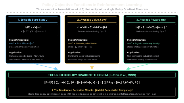
Policy gradient methods define scalar objective functions measuring policy performance across episodic, average value, and continuous average reward settings.
Why Does This Exist?
In value-based reinforcement learning (such as Q-learning or DQN), the learning goal is implicit: minimize Bellman error until the action-value function converges to .
In policy-based methods, however, the agent directly optimizes a parameterized policy via gradient ascent:
To compute that gradient, we must define the scalar performance objective being maximized. In real-world reinforcement learning, problems exhibit fundamentally different temporal horizons:
- Episodic tasks that naturally terminate at a terminal goal or timeout (games, robotic grasping).
- Continuing discounted tasks where an ongoing process is evaluated across stationary state visitations with time-preference discounting (server load balancing).
- Continuing undiscounted tasks where an infinite-horizon process runs indefinitely and success is measured purely by steady-state throughput (chemical refining, continuous industrial heating, high-frequency trading).
Selecting the wrong objective distorts learning. Applying discounted objectives to continuing problems introduces artificial horizon truncation, while episodic objectives fail on open-ended streams.
Furthermore, defining appears to create a major theoretical dilemma: depends on both through action selection probabilities and through the resulting state distribution . Without a special mathematical structure, computing would require differentiating the environmental state transition dynamics —an intractable model-dependent quantity. Understanding policy objective functions reveals the central miracle of policy gradients: across all three formulations, cancels out entirely.
Think of It Like This
Performance Metrics for an Investment Portfolio Manager
Imagine evaluating the executive performance of an investment portfolio manager whose algorithmic trading parameters execute continuous financial allocations.
Depending on the fund's contractual charter, investors evaluate the manager using three distinct performance metrics:
-
Metric 1: Final Maturity Payout ( - Episodic Start-State Value): In a 5-year fixed-term venture fund starting with an initial capital deposit on Day 1 (), the manager is evaluated strictly on total accumulated wealth upon liquidation at Year 5. All interim quarterly valuations only matter insofar as they maximize total discounted return from start state .
-
Metric 2: Average Portfolio Net Asset Value ( - Continuing Average Value): In an ongoing wealth management trust with quarterly discounting, the trustee measures the expected account balance averaged across all quarters. The score weights bull, bear, and sideways market regimes by how frequently the portfolio naturally visits them ().
-
Metric 3: Steady-State Dividend Yield ( - Continuous Average Reward): In a perpetual endowment fund that never liquidates, investors care only about the steady-state cash flow generated per day (dividend yield rate ). Immediate fluctuations in principal are irrelevant; the sole objective is maximizing the sustainable dividend rate per unit time.
The unifying insight: Even though the three accounting metrics measure distinct financial horizons, the trades the manager must execute (buying undervalued assets and selling overvalued assets) share the exact same directional gradient.
Where the analogy stops: Financial markets suffer from non-stationary macro shocks; in reinforcement learning, the environment transition dynamics are stationary Markov Decision Processes governed by ergodic chains.
How It Actually Works
The Three Canonical Mathematical Formulations
1. Episodic Start-State Objective
In episodic environments with a designated start state , the objective is the expected discounted cumulative return from :
If the initial state is drawn from a starting distribution , the objective generalizes to the expectation over starting states:
Under this formulation, the state visitation distribution is the unnormalized discounted on-policy state visitation frequency:
2. Continuing Average Value Objective
In continuing environments evaluated with discount factor , we measure the average state value weighted by the stationary distribution :
Where is the stationary distribution under policy , satisfying the balance equations:
3. Continuous Average Reward Objective
In continuing environments without discounting (), accumulated returns diverge to infinity. The canonical metric is the average reward per time step (the reward rate ):
Where is the expected immediate reward.
The Unifying Policy Gradient Theorem
Differentiating any of these objectives appears daunting because the state distribution depends directly on policy parameters :
Evaluating would require knowing the environment's internal transition probabilities , making model-free learning impossible.
The Policy Gradient Theorem (Sutton et al., 1999) establishes that for all three objectives, the state distribution gradient miraculously vanishes:
Using the identity , this converts directly to an expectation over trajectory samples:
This single unifying result allows REINFORCE, Actor-Critic, PPO, and TRPO to optimize policies without modeling environmental dynamics.
Worked Numerical Example
Consider a 2-state cyclic MDP with states and discount factor :
- State 1: The agent chooses between:
- Action (Safe): Loops with reward .
- Action (Switch): Transitions with reward .
- State 2: Forced deterministic transition with reward .
- Policy parameter: Let be the probability of taking the Switch action in state 1.
1. Stationary Distribution
Transition probability matrix:
The stationary distribution satisfies . Since :
2. Continuous Average Reward Objective
Expected reward in State 1: . Expected reward in State 2: .
3. Episodic Start-State Value with
From State 2: . From State 1:
4. Continuing Average Value Objective
Numerical Evaluation Across Policy Values:
| Policy | Stationary | Episodic | Average Value | Average Reward |
|---|---|---|---|---|
| (Always Safe) | ||||
| (Balanced) | ||||
| (Always Switch) |
All three objective functions strictly increase as goes from , confirming that all three formulations agree on the optimal policy () while operating under distinct mathematical units.
Code
from typing import Dict, Tuple
def evaluate_policy_objectives( p: float, gamma: float = 0.8,) -> Dict[str, float]: """Compute analytical policy objective functions for the 2-state cyclic MDP.
Args: p: Probability of taking action a1 (Switch) in State 1. gamma: Discount factor for episodic and average value objectives.
Returns: Dictionary containing stationary distribution and all 3 objective values. """ if not 0.0 <= p <= 1.0: raise ValueError("Policy parameter p must be in [0, 1].")
# 1. Stationary Distribution: d1 = 1 / (1 + p), d2 = p / (1 + p) d1 = 1.0 / (1.0 + p) d2 = p / (1.0 + p)
# 2. Continuous Average Reward Objective: J_avR = (1 + 2p) / (1 + p) j_avr = (1.0 + 2.0 * p) / (1.0 + p)
# 3. Episodic Start-State Objective: J_1 = V(1) = (1 + 2p) / (0.2 + 0.16p) # Derived from Bellman system: V(2) = gamma * V(1) denom = (1.0 - gamma) + p * gamma * (1.0 - gamma) v1 = (1.0 + 2.0 * p) / (denom) v2 = gamma * v1
# 4. Continuing Average Value Objective: J_avV = d1 * V(1) + d2 * V(2) j_avv = d1 * v1 + d2 * v2
return { "d1": d1, "d2": d2, "J_1": v1, "J_avV": j_avv, "J_avR": j_avr, }
def simulate_empirical_average_reward(p: float, steps: int = 100_000) -> float: """Empirical Monte Carlo rollout verifying continuous average reward r(pi).""" import random
random.seed(3) state = 1 total_reward = 0.0
for _ in range(steps): if state == 1: action = 1 if random.random() < p else 0 if action == 0: reward = 1.0 state = 1 else: reward = 3.0 state = 2 else: # state == 2 reward = 0.0 state = 1 total_reward += reward
return total_reward / steps
if __name__ == "__main__": test_policies = [0.0, 0.5, 1.0]
print("Policy (p) | d(s) = [d1, d2] | J_1 (Start) | J_avV (Avg Val) | J_avR (Avg Reward)") print("-" * 76)
for p in test_policies: res = evaluate_policy_objectives(p, gamma=0.8) print( f" p = {p:3.1f} | [{res['d1']:.4f}, {res['d2']:.4f}] | {res['J_1']:7.4f} |" f" {res['J_avV']:7.4f} | {res['J_avR']:7.4f}" )
# Validate empirical simulation against analytical average reward for p=0.5 empirical_r = simulate_empirical_average_reward(p=0.5, steps=100_000) print(f"\nEmpirical Monte Carlo Average Reward (p=0.5): {empirical_r:.4f}") print(f"Analytical Continuous Average Reward (p=0.5): 1.3333")# Expected Output:# Policy (p) | d(s) = [d1, d2] | J_1 (Start) | J_avV (Avg Val) | J_avR (Avg Reward)# ----------------------------------------------------------------------------# p = 0.0 | [1.0000, 0.0000] | 5.0000 | 5.0000 | 1.0000# p = 0.5 | [0.6667, 0.3333] | 7.1429 | 6.6667 | 1.3333# p = 1.0 | [0.5000, 0.5000] | 8.3333 | 7.5000 | 1.5000# # Empirical Monte Carlo Average Reward (p=0.5): 1.3333# Analytical Continuous Average Reward (p=0.5): 1.3333Watch Out For
The Continuing Task Discounting Paradox
A pervasive trap in reinforcement learning is applying the discounted episodic objective () to continuing, infinite-horizon tasks that lack an absorbing terminal state.
As Sutton & Barto (2018, Section 10.4) emphasize, using discounting in non-terminating tasks creates an artificial horizon bias:
- Time-Preference Distortion: The agent prioritizes immediate short-term payoffs over long-term sustainable throughput, even when the task runs forever.
- Distribution Mismatch: The discounted state distribution depends heavily on the arbitrary choice of and does not match the true stationary distribution .
The Fix: For true continuing, non-terminating tasks, use the Average Reward formulation () with undiscounted differential returns:
Differential returns measure performance relative to the steady-state baseline reward rate, eliminating artificial discounting bias while maintaining mathematical convergence.
The Quick Version
- Three Canonical Metrics: Performance is formalized via Episodic Start-State Value (), Continuing Average Value (), or Continuous Average Reward ().
- The Policy Gradient Miracle: The Policy Gradient Theorem proves that the gradient of the state distribution cancels out across all three formulations, enabling model-free optimization.
- Match Horizon to Objective: Use episodic objectives for tasks with designated start and termination states; use average reward formulations for continuing infinite-horizon industrial processes.
- Avoid False Discounting: Discounting in continuing tasks introduces artificial horizon truncation; true non-terminating control requires differential returns anchored to the average reward rate.