Policy in Reinforcement Learning

Why Does This Exist?

In reinforcement learning, an agent does not follow hardcoded rules or step-by-step procedures. Instead, it must decide what action to take in response to whatever situation it encounters. The policy ($\pi$) is the mathematical formalization of that decision mechanism: the mapping from perceived states of the environment to actions.

Without a formally defined policy, reinforcement learning collapses:

• No distinction between evaluation and execution: In value-based methods, an agent evaluates states using value functions ($V(s)$ or $Q(s, a)$), but an evaluation is not an action. A value function tells the agent how good a situation is, whereas a policy specifies what to actually do.
• No framework for exploration: If an agent only possessed fixed actions, it could never systematically balance exploring untried behaviors against exploiting known successes. A stochastic policy allows controlled randomness that can be tuned as learning progresses.
• No target for policy optimization: Direct policy methods like Policy Gradient Methods optimize the parameters of a policy function directly using gradient ascent. Without a formal policy representation, policy gradient algorithms cannot be derived.

A policy is the central entity in Markov Decision Processes. While models predict how the environment responds and value functions predict the accumulated return, the policy is the actor itself.

Think of It Like This

How It Actually Works

Deterministic vs. stochastic policy formulations

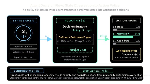
A policy can take two fundamental mathematical forms depending on whether action selection is certain or probabilistic.

1Deterministic Policy:    State s ──────► [ μ(s) ] ──────► Single Action a2Stochastic Policy:       State s ──────► [ π(a|s) ] ─────► Probability Distribution P(A=a|S=s)

1. Deterministic policies ($\mu$)

A deterministic policy is a direct mapping from the state space $\mathcal{S}$ to the action space $\mathcal{A}$:

$\mu: \mathcal{S} \to \mathcal{A}, \quad a = \mu(s)$

Given state $s$, the agent always selects the identical action $a$. Deterministic policies are common in continuous control tasks (such as robotic joint torque control in algorithms like DDPG and TD3) and during test-time evaluation when exploration is disabled.

2. Stochastic policies ($\pi$)

A stochastic policy defines a conditional probability distribution over actions given the current state:

$\pi: \mathcal{S} \times \mathcal{A} \to [0, 1], \quad \pi(a \mid s) = \mathbb{P}(A_t = a \mid S_t = s)$

For any valid stochastic policy over a discrete action space, two axioms must hold:

1. Non-negativity: $\pi(a \mid s) \ge 0$ for all $a \in \mathcal{A}$ and $s \in \mathcal{S}$.
2. Total probability: $\sum_{a \in \mathcal{A}} \pi(a \mid s) = 1$ for all $s \in \mathcal{S}$.

In continuous action spaces where $\mathcal{A} \subseteq \mathbb{R}^d$, $\pi(a \mid s)$ is a probability density function satisfying $\int_{\mathcal{A}} \pi(a \mid s)\, da = 1$. It is commonly parameterized as a Gaussian distribution $\mathcal{N}(\mu_\theta(s), \Sigma_\theta(s))$ whose mean and covariance are generated by neural networks.

3. Deriving policies from value functions

In value-based reinforcement learning, agents learn state-action values $Q(s, a)$ and derive policies from them:

• Greedy policy: Selects the action with the highest estimated value: $\pi_{\text{greedy}}(s) = \arg\max_{a \in \mathcal{A}} Q(s, a)$

• $\epsilon$-greedy policy: Balances exploitation with uniform random exploration: $\pi(a \mid s) = \begin{cases} 1 - \epsilon + \frac{\epsilon}{|\mathcal{A}|} & \text{if } a = \arg\max_{a'} Q(s, a') \\ \frac{\epsilon}{|\mathcal{A}|} & \text{otherwise} \end{cases}$

• Softmax (Boltzmann) policy: Converts action-values into probabilities proportional to their expected return using a temperature parameter $\tau > 0$: $\pi(a \mid s) = \frac{\exp(Q(s, a) / \tau)}{\sum_{b \in \mathcal{A}} \exp(Q(s, b) / \tau)}$

When $\tau \to \infty$, the distribution becomes uniform random (maximum exploration). When $\tau \to 0^+$, the distribution collapses to the deterministic greedy action (pure exploitation).

4. The optimal policy ($\pi^*$)

A policy $\pi^*$ is defined as optimal if its expected return from any state is greater than or equal to that of any other policy:

$V^{\pi^*}(s) \ge V^\pi(s) \quad \forall s \in \mathcal{S}, \; \forall \pi$

A foundational theorem of Markov Decision Processes states that for any MDP, there exists at least one stationary, deterministic policy that is globally optimal ($\pi^* = \mu^*$). Even though optimal policies in fully observable MDPs can be deterministic, stochastic policies remain essential during training to drive exploration and discover that optimum.

Worked numerical example

Consider an autonomous vehicle approaching a signalized intersection where the traffic light turns yellow.

• Observed state $s$: Distance to stop line $d = 30\text{ m}$, velocity $v = 45\text{ km/h}$, yellow duration elapsed $t = 1.2\text{ s}$.
• Available discrete actions:
  • $a_1$: Maintain current speed
  • $a_2$: Brake firmly
  • $a_3$: Accelerate through the yellow light
• Learned action values ($Q(s, a)$):
  • $Q(s, a_1) = 2.40$
  • $Q(s, a_2) = 1.10$
  • $Q(s, a_3) = 3.20$

Step 1: Deterministic greedy action selection

Under a deterministic greedy policy $\mu(s) = \arg\max_a Q(s, a)$:

$\mu(s) = \arg\max \{Q(s, a_1)=2.40, \; Q(s, a_2)=1.10, \; Q(s, a_3)=3.20\} = a_3$

The vehicle deterministically selects $a_3$ ("Accelerate").

Step 2: Stochastic Softmax policy calculation ($\tau = 1.0$)

To enable exploration, we compute the Boltzmann distribution at temperature $\tau = 1.0$:

1. Compute exponents: $\exp\left(\frac{Q(s, a_1)}{\tau}\right) = \exp(2.40) \approx 11.0232$ $\exp\left(\frac{Q(s, a_2)}{\tau}\right) = \exp(1.10) \approx 3.0042$ $\exp\left(\frac{Q(s, a_3)}{\tau}\right) = \exp(3.20) \approx 24.5325$

2. Sum the exponents to obtain the partition function $Z$: $Z = 11.0232 + 3.0042 + 24.5325 = 38.5599$

3. Calculate normalized action probabilities $\pi(a \mid s)$: $\pi(a_1 \mid s) = \frac{11.0232}{38.5599} \approx 0.2859 \quad (28.59\%)$ $\pi(a_2 \mid s) = \frac{3.0042}{38.5599} \approx 0.0779 \quad (7.79\%)$ $\pi(a_3 \mid s) = \frac{24.5325}{38.5599} \approx 0.6362 \quad (63.62\%)$

4. Verification of the total probability axiom: $0.2859 + 0.0779 + 0.6362 = 1.0000 \quad (100.00\%)$

Step 3: Temperature sensitivity comparison

The temperature parameter $\tau$ modulates the agent's exploration profile:

As $\tau \to 0$, action $a_3$ dominates ($93.46\% \to 100\%$). As $\tau$ increases, the probability mass flattens toward a uniform distribution ($\approx 33.33\%$ each), encouraging active exploration of lower-value actions.

Code

1from typing import List, Sequence, Tuple2import numpy as np3
4class PolicyEvaluator:5    """Demonstrates deterministic greedy and stochastic softmax policies."""6
7    def __init__(self, action_names: Sequence[str]) -> None:8        self.action_names = list(action_names)9        self.num_actions = len(action_names)10
11    def deterministic_greedy(self, q_values: np.ndarray) -> Tuple[int, str]:12        """Selects the action with the maximum Q-value.13
14        Args:15            q_values: 1D array of shape (num_actions,) containing expected returns.16
17        Returns:18            Tuple of (action_index, action_name).19        """20        action_idx = int(np.argmax(q_values))21        return action_idx, self.action_names[action_idx]22
23    def softmax_probabilities(24        self, q_values: np.ndarray, temperature: float = 1.025    ) -> np.ndarray:26        """Computes Boltzmann action probabilities with numerical stability.27
28        Args:29            q_values: 1D array of action values.30            temperature: Exploration parameter tau > 0.31
32        Returns:33            Normalized 1D probability distribution summing to 1.0.34        """35        if temperature <= 0:36            raise ValueError("Temperature tau must be strictly positive.")37
38        # Subtract max for numerical stability to prevent float overflow39        scaled_q = (q_values - np.max(q_values)) / temperature40        exp_q = np.exp(scaled_q)41        probabilities = exp_q / np.sum(exp_q)42        return probabilities43
44    def sample_stochastic(45        self, probabilities: np.ndarray, rng: np.random.Generator46    ) -> Tuple[int, str]:47        """Samples an action according to the probability distribution pi(a|s)."""48        action_idx = int(rng.choice(self.num_actions, p=probabilities))49        return action_idx, self.action_names[action_idx]50
51
52# Define intersection yellow light scenario53actions = ["Maintain Speed", "Brake firmly", "Accelerate"]54q_values = np.array([2.40, 1.10, 3.20], dtype=np.float64)55
56evaluator = PolicyEvaluator(actions)57rng = np.random.default_rng(seed=42)58
59# 1. Evaluate deterministic policy60det_idx, det_name = evaluator.deterministic_greedy(q_values)61print(f"Deterministic Greedy Policy:")62print(f"  Selected: {det_name} (Index {det_idx}) with Q = {q_values[det_idx]:.2f}\n")63
64# 2. Evaluate stochastic Softmax policy at tau = 1.065probs_standard = evaluator.softmax_probabilities(q_values, temperature=1.0)66print("Stochastic Policy Probabilities (tau = 1.0):")67for name, prob in zip(actions, probs_standard):68    print(f"  {name:<15}: {prob * 100:6.2f}%")69print(f"  Total Probability Sum: {np.sum(probs_standard):.4f}\n")70
71# 3. Simulate 10,000 empirical action samples72num_samples = 10_00073samples = [evaluator.sample_stochastic(probs_standard, rng)[0] for _ in range(num_samples)]74counts = np.bincount(samples, minlength=len(actions))75
76print(f"Empirical Frequencies from {num_samples:,} Samples:")77for name, count in zip(actions, counts):78    empirical_prob = (count / num_samples) * 10079    print(f"  {name:<15}: {count:5d} draws ({empirical_prob:5.2f}%)")

1Deterministic Greedy Policy:2  Selected: Accelerate (Index 2) with Q = 3.203
4Stochastic Policy Probabilities (tau = 1.0):5  Maintain Speed :  28.59%6  Brake firmly   :   7.79%7  Accelerate     :  63.62%8  Total Probability Sum: 1.00009
10Empirical Frequencies from 10,000 Samples:11  Maintain Speed :  2855 draws (28.55%)12  Brake firmly   :   781 draws ( 7.81%)13  Accelerate     :  6364 draws (63.64%)

Watch Out For

The Quick Version

• A policy ($\pi$) is the decision-making rule of an RL agent, mapping environmental states to actions to maximize cumulative reward.
• Deterministic policies ($a = \mu(s)$) output a single designated action per state; stochastic policies ($\pi(a \mid s)$) output a normalized probability distribution across the action space.
• While fully observable MDPs guarantee the existence of an optimal deterministic policy ($\pi^*$), stochastic policies are required during training to drive exploration and in POMDPs/games to avoid exploitable predictability.
• Value-based agents derive policies using greedy selection ($\arg\max_a Q(s, a)$), $\epsilon$-greedy exploration, or Boltzmann/Softmax distributions controlled by a temperature parameter $\tau$.

What to Read Next

• Markov Decision Processes
• Policy Gradient Methods
• Value Functions