Probabilistic Embeddings for Actor-Critic RL (PEARL)

PEARL figures out which task you are in from a handful of recent steps, then runs a task-aware SAC policy. One encoder, one policy, fast adaptation without new gradients.

PEARL infers a latent task variable z from recent context and conditions a SAC policy on it, sharpening from prior to posterior as evidence arrives.

Why Does This Exist?

Standard deep RL starts over on every new task. Change the goal velocity of a simulated cheetah from 1.0 m/s to 2.5 m/s and the old policy fails, so you burn millions more steps retraining from zero. That cost is painful when each environment step means a physics simulation or a real robot trial.

Meta-Reinforcement Learning promises a way out: train across a family of tasks so a new task takes a few episodes, not millions of steps. But the early answers were sample-hungry in their own way. Gradient based methods such as MAML in RL need fresh on-policy rollouts for every meta update, and recurrent black-box methods tangle the adaptation rule inside one memory network that is hard to reuse off policy.

PEARL, introduced by Rakelly and coauthors in 2019, takes an inference view instead. Keep one off-policy Soft Actor-Critic agent, add a context encoder that reads recent transitions and infers a compact task variable, then condition the policy and critic on that variable. Meta-training reuses old replay data like SAC does, and meta-testing adapts by updating a small belief, not by taking gradient steps through the whole policy.

This page teaches that inference loop: context to belief to task aware action. For the task family setup, start with the meta-RL page. For the entropy regularized actor critic underneath, read the SAC page. For the gradient step alternative, compare with the MAML page.

Think of It Like This

The Substitute Chef Who Tastes First

You walk in as the substitute chef in a busy kitchen you have never worked in. The menu says there are two house regulars: one orders extra salt, the other orders no salt. Nobody tells you which regular is at table six tonight.

You do not re-read the whole cookbook. You taste three spoonfuls from tonight's pot. Spoon one is fairly salty, spoon two is very salty, spoon three is mildly salty. Your palate averages the evidence and you write one recipe card: tonight's kitchen runs salty, strength about 0.9 out of 1. You clip that card to your station and cook the whole dinner service from it, reaching for salt with confidence.

Next night the spoonfuls taste flat. Same averaging, opposite verdict: card says low salt, and your hands adjust without relearning how to chop or stir.

Where it stops: a real palate is not a permutation invariant neural net, and no chef pays a KL penalty to keep the recipe card near a prior. The locking in matters though. You commit to one card for the whole service instead of second guessing after every bite, which is exactly what posterior sampling does for an episode.

How It Actually Works

PEARL has three moving parts: a context, a probabilistic encoder, and SAC networks that listen to the encoder's sample.

A task $\mathcal{T}$ is one MDP drawn from a task distribution $p(\mathcal{T})$ , the family of jobs you train across. Plain words: $p(\mathcal{T})$ is the menu of possible kitchens, and $\mathcal{T}$ is tonight's kitchen. A context $c$ is a small bag of recent transitions $(s, a, r, s^{\prime})$ , where $s$ is the state, $a$ is the action taken, $r$ is the reward received, and $s^{\prime}$ is the next state. The latent task variable $z$ is a short vector that summarizes which task the context points to. The encoder $q_{\phi}(z \mid c)$ maps a context to a distribution over $z$ , with weights $\phi$ . The policy $\pi_{\theta}(a \mid s, z)$ maps a state plus a task sample to an action distribution, with weights $\theta$ . The critic $Q(s, a, z)$ scores how good a state, action, and task guess are together.

Context encoder and conditioned SAC

Each transition passes through a shared small network $f_{\phi}$ , which outputs one Gaussian factor per transition. The encoder multiplies those factors with a standard normal prior $\mathcal{N}(0, I)$ and renormalizes, which for unit variance factors gives a clean product rule. The actor and critic are ordinary SAC networks with one change: they concatenate $z$ to their inputs.

Meta-training samples two batches per task from separate replay buffers: a context batch to infer $z$ and an RL batch for the Bellman update. The critic minimizes the soft Bellman error plus an information bottleneck $\beta \, \mathrm{KL}(q_{\phi}(z \mid c) \parallel \mathcal{N}(0, I))$ , where $\beta$ is a scalar that caps how much task detail $z$ may carry and $\mathrm{KL}$ measures distance from the prior. The actor maximizes the SAC objective with its entropy bonus weighted by temperature $\alpha$ . The encoder learns through the critic loss only, never through the actor loss, because actor gradients proved too noisy in the paper's ablations.

Meta-testing needs no gradients. At the start of each episode, sample one $z$ from the current posterior $q_{\phi}(z \mid c)$ and hold it fixed for the whole episode. That fixed sample is posterior sampling, also called Thompson sampling: with an empty context you draw from the broad prior and try something coherent, and as context piles up the posterior sharpens and your behavior locks onto the identified task. Per step noise would dither; per episode commitment explores.

Worked example: three transitions to one action

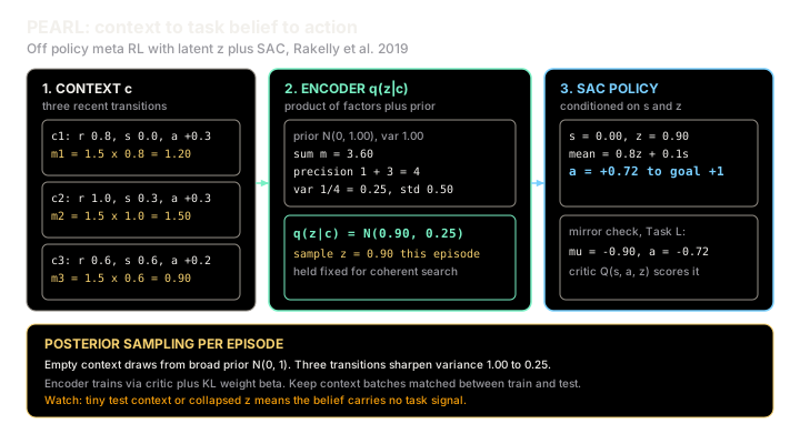
Take a 1D line with two tasks. Task R has its goal at $+1$ , Task L has its goal at $-1$ . The agent sits at $s = 0.0$ in a new episode and holds three context transitions from earlier probing that all moved right and earned positive reward:

$c_1 = (s=0.0, a=+0.3, r=0.8), \quad c_2 = (s=0.3, a=+0.3, r=1.0), \quad c_3 = (s=0.6, a=+0.2, r=0.6)$

Use a toy encoder where each factor mean is $m_i = 1.5 \times r_i$ . Then:

$m_1 = 1.5 \times 0.8 = 1.20, \quad m_2 = 1.5 \times 1.0 = 1.50, \quad m_3 = 1.5 \times 0.6 = 0.90$

Sum the factors to get $3.60$ . The prior contributes precision $1$ and each of the three factors contributes precision $1$ , so total precision is $1 + 3 = 4$ . Posterior variance is $1 / 4 = 0.25$ with standard deviation $0.50$ , down from the prior variance $1.00$ . Posterior mean is $3.60 / 4 = 0.90$ . So:

$q(z \mid c) = \mathcal{N}(0.90, \, 0.25)$

Sample the mean $z = 0.90$ for this episode. The toy conditioned policy uses mean action $\mu_a = 0.8 \times z + 0.1 \times s$ . At $s = 0.0$ :

$\mu_a = 0.8 \times 0.90 + 0.1 \times 0.0 = 0.72$

The agent steps about $+0.72$ toward the $+1$ goal. Had the context come from Task L with rewards $[-0.8, -1.0, -0.6]$ , the same math gives $\mu = -0.90$ and mean action $-0.72$ toward $-1$ . The diagram draws this exact chain: three rewards to one belief to one rightward action. The KL cost of this belief against the prior is about $0.72$ nats before weighting by $\beta$ , which is the price of carrying task detail.

Code

The snippet below replays the worked numbers: encode three rewards into a Gaussian belief, condition a toy policy mean on the sample, and check both task directions.

1from dataclasses import dataclass2
3
4@dataclass5class PearlPosterior:6    mu: float7    var: float8
9
10def encode_context(rewards: list[float], factor_scale: float = 1.5) -> PearlPosterior:11    """Product of unit-variance Gaussian factors plus a standard normal prior."""12    total = sum(factor_scale * r for r in rewards)13    precision = 1.0 + len(rewards)14    return PearlPosterior(mu=total / precision, var=1.0 / precision)15
16
17def policy_mean_action(z: float, s: float = 0.0) -> float:18    """Toy conditioned policy mean: 0.8 * z + 0.1 * s."""19    return 0.8 * z + 0.1 * s20
21
22def main() -> None:23    right = [0.8, 1.0, 0.6]24    q = encode_context(right)25    a = policy_mean_action(q.mu, s=0.0)26    print(f"posterior mu={q.mu:.2f} var={q.var:.2f} action={a:.2f}")27    left = [-0.8, -1.0, -0.6]28    ql = encode_context(left)29    al = policy_mean_action(ql.mu, s=0.0)30    print(f"left mu={ql.mu:.2f} var={ql.var:.2f} action={al:.2f}")31    assert abs(q.mu - 0.9) < 1e-932    assert abs(q.var - 0.25) < 1e-933    assert abs(a - 0.72) < 1e-934    print("checks passed")35
36
37if __name__ == "__main__":38    main()

1# -> expected output:2posterior mu=0.90 var=0.25 action=0.723left mu=-0.90 var=0.25 action=-0.724checks passed

Watch Out For

Testing on a context the encoder never saw

The symptom is familiar: meta-training curves look healthy, then the new task adapts slowly or picks the wrong direction for several episodes. The usual cause is context shift. Training sampled large uniform context batches of a few hundred transitions, while testing feeds the last five online steps, or vice versa. The encoder learned one context size and distribution and now faces another, so its mean lands between tasks and the variance stays wide.

Fix it by matching the pipeline. Sample context batches the same size at train and test time, mix recent and uniform transitions the way the paper's sampler does, and keep the context batch separate from the RL batch. Log posterior mean and variance on held-out tasks during training. If the variance on new tasks sits far above training variance, your context pipeline drifted.

z-collapse: the policy stops listening to z

The symptom is a flat latent space. Posterior means hover near zero for every task, variances sit at the prior, and the policy takes the same actions whether the true goal is left or right. Two forces cause it: a bottleneck weight $\beta$ set so high that any nonzero $z$ costs more than it earns, or encoder gradients flowing through the actor loss, which drowns the task signal in policy noise.

Fix it the paper's way. Train the encoder through the critic loss only, start $\beta$ small and raise it until task separation just holds, and plot $z$ means colored by true task. Distinct clusters mean the encoder carries signal. One blob means you tuned the bottleneck shut. When in doubt, lower $\beta$ first and recheck the clusters before touching the network size.

The Quick Version

PEARL adds a context encoder to SAC so one policy serves a whole task family by conditioning on a latent task variable $z$ .
The encoder turns a bag of recent transitions into a Gaussian belief $q(z \mid c)$ , and each new episode samples one $z$ and holds it fixed for coherent exploration.
Off-policy replay buffers supply separate context and RL batches, which keeps sample cost far below on-policy meta-RL that needs fresh rollouts per update.
In the toy chain, rewards $[0.8, 1.0, 0.6]$ give posterior $\mathcal{N}(0.90, 0.25)$ and mean action $+0.72$ toward the right goal.
Context shift and $z$ -collapse are the two failures to check first when adaptation stalls or ignores the task.