Model-Agnostic Meta-Learning (MAML) in RL

Why Does This Exist?

Standard deep reinforcement learning algorithms are notoriously sample-inefficient. Training a robotic arm to grasp a specific cup or teaching an autonomous car to navigate a single intersection can require millions of environment interactions. If the task changes slightly—such as changing the friction of the floor, altering the target speed, or switching to an object with different mass—standard RL algorithms must restart learning from scratch or undergo extensive retraining.

Meta-Reinforcement Learning addresses this challenge by framing learning at the task level: given a family of related tasks $\mathcal{T} \sim p(\mathcal{T})$, the agent aims to "learn how to learn" so that it can adapt to a novel, unseen task $\mathcal{T}_{\text{new}}$ using only a handful of exploratory trials.

Early Meta-RL architectures relied primarily on black-box recurrent networks (such as RL²). In these models, a recurrent network (LSTM or GRU) ingests past trajectories, rewards, and actions into its hidden state $h_t$, effectively executing an internal adaptation algorithm inside memory. However, recurrent black-box Meta-RL methods face steep challenges:

1. Difficult Generalization: When presented with tasks outside the narrow training distribution, recurrent policies cannot leverage gradient-based updates to adapt further.
2. Architecture Entanglement: The adaptation mechanism is tightly bound to a specific recurrent architecture, making it difficult to swap in state-of-the-art policy architectures.

In 2017, Chelsea Finn, Pieter Abbeel, and Sergey Levine introduced Model-Agnostic Meta-Learning (MAML). Instead of embedding adaptation into recurrent activations, MAML grounds adaptation in gradient descent itself. MAML seeks an initial policy parameter vector $\theta$ that is not necessarily optimal for any single task, but maximally sensitive to the loss landscapes of all tasks in $p(\mathcal{T})$. Consequently, taking just one or two standard policy gradient steps on a small batch of rollouts propels the policy directly to high performance on that new task.

Think of It Like This

How It Actually Works

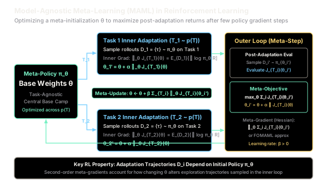
MAML optimizes a parameterized policy $\pi_\theta(a \mid s)$ over a distribution of tasks $\mathcal{T}_i \sim p(\mathcal{T})$. The optimization operates in a nested bi-level structure: an Inner Loop that adapts to a specific task, and an Outer Loop that optimizes the initial weights across all tasks.

1                    Meta-Policy Base Weights θ2                                │3         ┌──────────────────────┴──────────────────────┐4         ▼                                             ▼5┌───────────────────────────────┐             ┌───────────────────────────────┐6│ Task 1 Inner Adaptation (T_1) │             │ Task 2 Inner Adaptation (T_2) │7│ 1. Collect D_1 ~ π_θ          │             │ 1. Collect D_2 ~ π_θ          │8│ 2. Compute ∇_θ J_{T_1}(θ)     │             │ 2. Compute ∇_θ J_{T_2}(θ)     │9│ 3. θ_1' = θ + α ∇ J_{T_1}(θ)  │             │ 3. θ_2' = θ + α ∇ J_{T_2}(θ)  │10└───────────────┬───────────────┘             └───────────────┬───────────────┘11                │                                             │12                ▼                                             ▼13        Adapted Policy π_{θ_1'}                       Adapted Policy π_{θ_2'}14        Evaluate on T_1: J_{T_1}(θ_1')                Evaluate on T_2: J_{T_2}(θ_2')15                │                                             │16                └──────────────────────┬──────────────────────┘17                                       ▼18                         ┌───────────────────────────┐19                         │ Outer Loop Meta-Objective │20                         │ max_θ Σ_i J_{T_i}(θ_i')   │21                         └─────────────┬─────────────┘22                                       │23                                       ▼ (Meta-Gradient Step)24                         θ ← θ + β Σ_i ∇_θ J_{T_i}(θ_i')

The Inner Loop: Task-Specific Policy Adaptation

For a sampled task $\mathcal{T}_i \sim p(\mathcal{T})$:

1. The agent uses the current meta-policy $\pi_\theta$ to collect a small set of rollout trajectories $\mathcal{D}_i = \{\tau^{(j)}\}$, where $\tau = (s_0, a_0, r_0, \dots, s_T)$.
2. The agent computes the task-specific policy gradient:

$\nabla_\theta J_{\mathcal{T}_i}(\theta) = \mathbb{E}_{\tau \sim \pi_\theta} \left[ \sum_{t=0}^T \nabla_\theta \log \pi_\theta(a_t \mid s_t) R_t(\tau) \right]$

3. The parameters are updated using a single (or few) policy gradient ascent steps with inner learning rate $\alpha$:

$\theta_i' = \theta + \alpha \nabla_\theta J_{\mathcal{T}_i}(\theta)$

The adapted parameter $\theta_i'$ defines a specialized task policy $\pi_{\theta_i'}$.

The Outer Loop: Meta-Gradient Optimization

To measure how well the initialization $\theta$ facilitated fast learning, MAML samples a fresh batch of validation trajectories $\mathcal{D}_i'$ on task $\mathcal{T}_i$ using the adapted policy $\pi_{\theta_i'}$.

The meta-objective maximizes the expected post-adaptation performance across all tasks:

$\mathcal{J}_{\text{meta}}(\theta) = \sum_{\mathcal{T}_i \sim p(\mathcal{T})} J_{\mathcal{T}_i}(\theta_i') = \sum_{\mathcal{T}_i \sim p(\mathcal{T})} J_{\mathcal{T}_i}\left( \theta + \alpha \nabla_\theta J_{\mathcal{T}_i}(\theta) \right)$

Applying the multivariate chain rule to update $\theta$ with meta-learning rate $\beta$:

$\theta \leftarrow \theta + \beta \sum_{\mathcal{T}_i \sim p(\mathcal{T})} \nabla_\theta J_{\mathcal{T}_i}(\theta_i')$

where the gradient of the post-adaptation return with respect to the initial parameters $\theta$ is:

$\nabla_\theta J_{\mathcal{T}_i}(\theta_i') = \nabla_{\theta_i'} J_{\mathcal{T}_i}(\theta_i') \cdot \frac{d \theta_i'}{d \theta} = \nabla_{\theta_i'} J_{\mathcal{T}_i}(\theta_i') \cdot \left( I + \alpha \nabla_\theta^2 J_{\mathcal{T}_i}(\theta) \right)$

The term $\nabla_\theta^2 J_{\mathcal{T}_i}(\theta)$ is the Hessian of the expected task return, making standard MAML a second-order optimization algorithm.

The RL-Specific Credit Assignment Dilemma

A crucial theoretical distinction exists between applying MAML in supervised learning versus reinforcement learning:

In supervised learning, the training dataset $\mathcal{D}_i$ is fixed and independent of model parameters. In reinforcement learning, however, the adaptation trajectories $\mathcal{D}_i$ are gathered by policy $\pi_\theta$ interacting with the environment:

$P(\tau \mid \theta) = p(s_0) \prod_{t=0}^T \pi_\theta(a_t \mid s_t) p(s_{t+1} \mid s_t, a_t)$

Because the distribution of trajectories depends directly on $\theta$, the true meta-gradient contains an additional exploration term:

$\nabla_\theta \mathbb{E}_{\tau \sim \pi_\theta} [\dots]$

This means MAML in RL not only optimizes initial parameters for fast adaptation, but also optimizes $\pi_\theta$ to explore effectively during the first trial to collect informative adaptation data!

Because computing exact second-order Hessians on noisy policy gradients causes extreme variance, practitioners frequently use First-Order MAML (FOMAML), which sets $\frac{d \theta_i'}{d \theta} \approx I$:

$\nabla_\theta \mathcal{J}_{\text{meta}}^{\text{FOMAML}}(\theta) \approx \sum_{\mathcal{T}_i} \nabla_{\theta_i'} J_{\mathcal{T}_i}(\theta_i')$

Worked numerical example

Let us trace the complete inner adaptation and outer meta-gradient update using a concrete 1D linear policy.

Step 1: Environment and Setup

Consider an agent learning a 1D linear policy $\pi_\theta(a \mid s) = \theta \cdot s$.

• State: $s = 1.0$.
• Two tasks with different target gains: Task 1 ($\mathcal{T}_1$: target slope $k_1 = 2.0$) and Task 2 ($\mathcal{T}_2$: target slope $k_2 = 4.0$).
• Reward function: quadratic negative error $r_i(\theta) = -(\theta \cdot s - k_i)^2$.
• Inner learning rate $\alpha = 0.10$, outer meta-learning rate $\beta = 0.10$.
• Current meta-initialization: $\theta = 2.50$.

Step 2: Task 1 Inner Adaptation

• Zero-shot reward on Task 1: $r_1 = -(2.50 \times 1.0 - 2.0)^2 = -(0.50)^2 = -0.2500$
• Task 1 policy gradient: $\nabla_\theta r_1 = -2(\theta \cdot s - 2.0) \cdot s = -2(2.50 - 2.0)(1.0) = -1.0000$
• 1-step inner adaptation: $\theta_1' = \theta + \alpha \nabla_\theta r_1 = 2.50 + 0.10(-1.0000) = 2.4000$
• Post-adaptation reward on Task 1: $r_1' = -(2.40 \times 1.0 - 2.0)^2 = -(0.40)^2 = -0.1600 \quad (\text{improved from } -0.2500)$

Step 3: Task 2 Inner Adaptation

• Zero-shot reward on Task 2: $r_2 = -(2.50 \times 1.0 - 4.0)^2 = -(-1.50)^2 = -2.2500$
• Task 2 policy gradient: $\nabla_\theta r_2 = -2(2.50 - 4.0)(1.0) = +3.0000$
• 1-step inner adaptation: $\theta_2' = \theta + \alpha \nabla_\theta r_2 = 2.50 + 0.10(+3.0000) = 2.8000$
• Post-adaptation reward on Task 2: $r_2' = -(2.80 \times 1.0 - 4.0)^2 = -(-1.20)^2 = -1.4400 \quad (\text{improved from } -2.2500)$

Step 4: Outer Loop Meta-Gradient Update

Total post-adaptation return across tasks: $\mathcal{J}_{\text{meta}}(\theta) = r_1' + r_2' = -0.1600 + (-1.4400) = -1.6000$ Notice this is substantially higher than the zero-shot return: $\mathcal{J}_{\text{zero-shot}}(\theta) = -0.2500 + (-2.2500) = -2.5000$

Now evaluate the full meta-gradient $\nabla_\theta \mathcal{J}_{\text{meta}}$:

• For Task 1: $\theta_1' = \theta - 0.2(\theta - 2.0) = 0.8\theta + 0.4 \implies \frac{d\theta_1'}{d\theta} = 0.80$. $\frac{d r_1'}{d\theta} = \frac{d r_1'}{d\theta_1'} \cdot \frac{d\theta_1'}{d\theta} = -2(2.40 - 2.0)(1.0) \times 0.80 = -0.80 \times 0.80 = -0.6400$
• For Task 2: $\theta_2' = \theta - 0.2(\theta - 4.0) = 0.8\theta + 0.8 \implies \frac{d\theta_2'}{d\theta} = 0.80$. $\frac{d r_2'}{d\theta} = \frac{d r_2'}{d\theta_2'} \cdot \frac{d\theta_2'}{d\theta} = -2(2.80 - 4.0)(1.0) \times 0.80 = +2.40 \times 0.80 = +1.9200$
• Total meta-gradient: $\nabla_\theta \mathcal{J}_{\text{meta}}(\theta) = -0.6400 + 1.9200 = +1.2800$
• Meta-update step: $\theta_{\text{new}} = \theta + \beta \nabla_\theta \mathcal{J}_{\text{meta}}(\theta) = 2.50 + 0.10(+1.2800) = 2.6280$

The base parameter $\theta$ successfully shifted from $2.50$ toward $2.628$ (moving toward the optimal midpoint $3.0$), making both tasks even easier to adapt to in future iterations!

Code

Below is a self-contained, typed Python implementation of MAMLReinforcementLearning demonstrating inner task adaptation, outer meta-gradient computation, and empirical return validation.

1import math2from typing import List, Tuple3
4
5class MAMLReinforcementLearning:6    """Simulates Model-Agnostic Meta-Learning (MAML) for a 1D policy across a family of tasks."""7
8    def __init__(self, alpha: float = 0.10, beta: float = 0.10) -> None:9        self.alpha = alpha  # Inner loop adaptation rate10        self.beta = beta  # Outer loop meta-learning rate11
12    def compute_task_reward(13        self, theta: float, target_k: float, s: float = 1.014    ) -> float:15        """Computes quadratic negative error reward: r = - (theta * s - k)^2."""16        pred = theta * s17        return -((pred - target_k) ** 2)18
19    def compute_inner_gradient(20        self, theta: float, target_k: float, s: float = 1.021    ) -> float:22        """Computes d(reward)/d(theta) = - 2 * (theta * s - k) * s."""23        return -2.0 * (theta * s - target_k) * s24
25    def inner_adaptation(26        self, theta: float, target_k: float, s: float = 1.027    ) -> Tuple[float, float, float, float]:28        """Performs 1-step inner policy gradient ascent on task target_k.29
30        theta' = theta + alpha * grad.31        Returns: (initial_reward, grad, theta_adapted, adapted_reward).32        """33        r_init = self.compute_task_reward(theta, target_k, s)34        grad = self.compute_inner_gradient(theta, target_k, s)35        theta_adapted = theta + self.alpha * grad36        r_adapted = self.compute_task_reward(theta_adapted, target_k, s)37        return r_init, grad, theta_adapted, r_adapted38
39    def meta_gradient_step(40        self, theta: float, tasks: List[float], s: float = 1.041    ) -> Tuple[float, float, float, float]:42        """Computes full second-order meta-gradient and performs meta-update."""43        total_meta_grad = 0.044        total_r_init = 0.045        total_r_adapted = 0.046
47        for k in tasks:48            r_init, _, theta_prime, r_adapt = self.inner_adaptation(49                theta, k, s50            )51            total_r_init += r_init52            total_r_adapted += r_adapt53
54            d_theta_prime_d_theta = 1.0 - 2.0 * self.alpha * (s**2)55            d_r_d_theta_prime = -2.0 * (theta_prime * s - k) * s56            meta_grad_i = d_r_d_theta_prime * d_theta_prime_d_theta57            total_meta_grad += meta_grad_i58
59        theta_new = theta + self.beta * total_meta_grad60        return total_r_init, total_r_adapted, total_meta_grad, theta_new61
62
63if __name__ == "__main__":64    maml = MAMLReinforcementLearning(alpha=0.10, beta=0.10)65
66    theta_0 = 2.5067    tasks = [2.0, 4.0]  # Task 1: target=2.0, Task 2: target=4.068    s = 1.069
70    # 1. Task 1 Evaluation71    r1_init, g1, theta1_p, r1_adapt = maml.inner_adaptation(theta_0, 2.0, s)72    print("=== Task 1 (Target k=2.0) ===")73    print(f"Zero-shot reward r_1:       {r1_init:.4f} (-(2.5 - 2.0)^2 = -0.2500)")74    print(f"Inner gradient:             {g1:.4f} (-2 * 0.5 * 1.0 = -1.0000)")75    print(f"Adapted parameter theta_1': {theta1_p:.4f} (2.5 + 0.1 * (-1.0) = 2.4000)")76    print(f"Adapted reward r_1':        {r1_adapt:.4f} (-(2.4 - 2.0)^2 = -0.1600)")77
78    assert math.isclose(r1_init, -0.2500)79    assert math.isclose(g1, -1.0000)80    assert math.isclose(theta1_p, 2.4000)81    assert math.isclose(r1_adapt, -0.1600)82
83    # 2. Task 2 Evaluation84    r2_init, g2, theta2_p, r2_adapt = maml.inner_adaptation(theta_0, 4.0, s)85    print("\n=== Task 2 (Target k=4.0) ===")86    print(f"Zero-shot reward r_2:       {r2_init:.4f} (-(2.5 - 4.0)^2 = -2.2500)")87    print(f"Inner gradient:             {g2:.4f} (-2 * (-1.5) * 1.0 = +3.0000)")88    print(f"Adapted parameter theta_2': {theta2_p:.4f} (2.5 + 0.1 * (+3.0) = 2.8000)")89    print(f"Adapted reward r_2':        {r2_adapt:.4f} (-(2.8 - 4.0)^2 = -1.4400)")90
91    assert math.isclose(r2_init, -2.2500)92    assert math.isclose(g2, 3.0000)93    assert math.isclose(theta2_p, 2.8000)94    assert math.isclose(r2_adapt, -1.4400)95
96    # 3. Outer Loop Meta-Update97    tot_init, tot_adapt, meta_grad, theta_next = maml.meta_gradient_step(98        theta_0, tasks, s99    )100    print("\n=== Meta-Objective & Outer Loop Update ===")101    print(f"Total Zero-shot return:     {tot_init:.4f} (-0.25 + -2.25 = -2.5000)")102    print(f"Total Post-adaptation return: {tot_adapt:.4f} (-0.16 + -1.44 = -1.6000)")103    print(f"Meta-gradient sum:          {meta_grad:.4f} (-0.64 + 1.92 = +1.2800)")104    print(f"Updated meta-param theta:   {theta_next:.4f} (2.50 + 0.10 * 1.28 = 2.6280)")105
106    assert math.isclose(tot_init, -2.5000)107    assert math.isclose(tot_adapt, -1.6000)108    assert math.isclose(meta_grad, 1.2800)109    assert math.isclose(theta_next, 2.6280)110    assert tot_adapt > tot_init111
112    print("\nAll MAML in RL simulation assertions passed successfully!")

Expected output:

1=== Task 1 (Target k=2.0) ===2Zero-shot reward r_1:       -0.2500 (-(2.5 - 2.0)^2 = -0.2500)3Inner gradient:             -1.0000 (-2 * 0.5 * 1.0 = -1.0000)4Adapted parameter theta_1': 2.4000 (2.5 + 0.1 * (-1.0) = 2.4000)5Adapted reward r_1':        -0.1600 (-(2.4 - 2.0)^2 = -0.1600)6
7=== Task 2 (Target k=4.0) ===8Zero-shot reward r_2:       -2.2500 (-(2.5 - 4.0)^2 = -2.2500)9Inner gradient:             3.0000 (-2 * (-1.5) * 1.0 = +3.0000)10Adapted parameter theta_2': 2.8000 (2.5 + 0.1 * (+3.0) = 2.8000)11Adapted reward r_2':        -1.4400 (-(2.8 - 4.0)^2 = -1.4400)12
13=== Meta-Objective & Outer Loop Update ===14Total Zero-shot return:     -2.5000 (-0.25 + -2.25 = -2.5000)15Total Post-adaptation return: -1.6000 (-0.16 + -1.44 = -1.6000)16Meta-gradient sum:          1.2800 (-0.64 + 1.92 = +1.2800)17Updated meta-param theta:   2.6280 (2.50 + 0.10 * 1.28 = 2.6280)18
19All MAML in RL simulation assertions passed successfully!

Watch Out For

The Quick Version

• Bi-Level Optimization: MAML separates learning into an inner loop (quick task-specific policy adaptation $\theta_i' = \theta + \alpha \nabla J_i(\theta)$) and an outer loop (meta-gradient update of base weights $\theta \leftarrow \theta + \beta \sum \nabla_\theta J_i(\theta_i')$).
• Model-Agnostic Flexibility: Because adaptation relies exclusively on standard gradient ascent, MAML can be applied to any differentiable policy architecture (MLPs, CNNs, Transformers) without specialized recurrent memory.
• Active Exploration Optimization: In reinforcement learning, the adaptation rollouts depend on the base policy $\pi_\theta$. MAML naturally trains the initial policy to gather diverse, informative trajectories during its first trial.
• First-Order Approximations: To mitigate the extreme variance and computational cost of second-order policy Hessians, practical implementations frequently leverage First-Order MAML (FOMAML) or trust-region proximal bounds (ProMP).

What to Read Next

• Meta-Reinforcement Learning
• Policy Gradient Methods
• Model-Based Deep RL