Meta-Reinforcement Learning

Why Does This Exist?

Traditional deep reinforcement learning is notoriously sample-inefficient. An agent trained to control a legged robot typically requires tens of millions of environmental simulation steps from scratch (tabula rasa) to master walking forward at a fixed velocity of 2.0 m/s.

Even worse, standard RL policies are brittle:

• If ground friction decreases by 15%, the robot slips and falls.
• If the goal velocity shifts to 3.5 m/s, the policy fails completely.
• To handle the modified environment, standard RL must re-initialize its networks and burn millions more samples relearning from zero.

Biological organisms never learn this way. A human learning a new sport does not restart cognitive development from infancy. Instead, humans draw upon prior motor foundations—balance, force modulation, spatial coordination—to master the rules of a new sport within minutes.

Meta-Reinforcement Learning (Meta-RL), or learning to learn, bridges this gap. Instead of optimizing a policy for a single, static Markov Decision Process (MDP), Meta-RL optimizes an agent across a broad distribution of tasks $p(\mathcal{T})$.

The fundamental goal is not to maximize performance during the initial exploratory interactions with a task. Rather, Meta-RL maximizes the agent's ability to rapidly adapt to an unseen test task $\mathcal{T}_{\text{test}} \sim p(\mathcal{T})$ using only one or a few exploratory trial episodes.

Think of It Like This

How It Actually Works

The Task Distribution Formulation

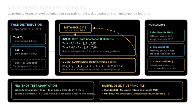
Meta-RL assumes a distribution over tasks $p(\mathcal{T})$. Each individual task $\mathcal{T}_i \sim p(\mathcal{T})$ is an MDP:

Typically, tasks in a distribution share state space $\mathcal{S}$ and action space $\mathcal{A}$, but vary in their transition dynamics $P_i(s' \mid s, a)$ (e.g., varying surface friction or leg damping) or reward functions $R_i(s, a)$ (e.g., navigating to different target coordinates).

The Bilevel Optimization Loop

Meta-RL solves a bilevel optimization problem that decouples fast adaptation from meta-training:

1. The Inner Loop (Fast Adaptation):
   • Given a task $\mathcal{T}_i \sim p(\mathcal{T})$ and base meta-parameters $\theta$, the agent rolls out exploratory trial episodes to collect a support dataset $\mathcal{D}_i^{\text{train}} \sim \pi_\theta$.
   • An adaptation operator updates $\theta$ into task-specific parameters $\theta_i'$. In gradient-based meta-learning, this is a standard policy gradient step: $$\theta_i' = \theta - \alpha \nabla_\theta \mathcal{L}_{\mathcal{T}_i}\left(\theta, \mathcal{D}_i^{\text{train}}\right)$$ where $\alpha$ is the inner-loop learning rate.
2. The Outer Loop (Meta-Optimization):
   • The adapted policy $\pi_{\theta_i'}$ is deployed in task $\mathcal{T}_i$ to collect a test query dataset $\mathcal{D}_i^{\text{test}} \sim \pi_{\theta_i'}$.
   • The outer loop computes the meta-objective, summing the loss of the adapted parameters across a batch of sampled tasks: $$\min_\theta \mathcal{L}_{\text{meta}}(\theta) = \mathbb{E}_{\mathcal{T}_i \sim p(\mathcal{T})} \left[ \mathcal{L}_{\mathcal{T}_i}\left(\theta_i', \mathcal{D}_i^{\text{test}}\right) \right]$$
   • The base meta-parameters $\theta$ are updated via meta-gradient descent: $$\theta \leftarrow \theta - \beta \nabla_\theta \sum_{\mathcal{T}_i} \mathcal{L}_{\mathcal{T}_i}\left(\theta_i', \mathcal{D}_i^{\text{test}}\right)$$ where $\beta$ is the outer-loop learning rate.

This bilevel structure forces the base parameters $\theta$ to settle into a representation from which any task $\mathcal{T}_i$ in the distribution is reachable within 1–3 gradient steps.

The Three Meta-RL Families

Practitioners implement fast adaptation through three distinct architectural paradigms:

Worked numerical example

Consider a 1D continuous velocity-tracking meta-environment where policies have state $s = 1.0$ and predict action $a = \theta \cdot s = \theta$.

We sample two training tasks from the distribution:

• Task 1 ($\mathcal{T}_1$): Target velocity $v_1^* = 2.0$.
• Task 2 ($\mathcal{T}_2$): Target velocity $v_2^* = 4.0$.

The task loss is squared tracking error: $\mathcal{L}_i(\theta) = \frac{1}{2}(\theta - v_i^*)^2$, with gradient $\nabla_\theta \mathcal{L}_i(\theta) = \theta - v_i^*$. Let the base meta-parameter be initialized at $\theta = 1.0000$. Inner learning rate $\alpha = 0.20$, outer meta-learning rate $\beta = 0.10$.

1. Inner Loop Fast Adaptation

• Task 1 ($v_1^* = 2.0$):
  • Gradient: $g_1 = \theta - v_1^* = 1.0000 - 2.0 = -1.0000$.
  • Adapted parameter: $$\theta_1' = \theta - \alpha g_1 = 1.0000 - 0.20(-1.0000) = 1.2000$$
• Task 2 ($v_2^* = 4.0$):
  • Gradient: $g_2 = \theta - v_2^* = 1.0000 - 4.0 = -3.0000$.
  • Adapted parameter: $$\theta_2' = \theta - \alpha g_2 = 1.0000 - 0.20(-3.0000) = 1.6000$$

2. Outer Loop Meta-Loss Evaluation

Evaluate the adapted parameters on each task:

• Task 1 post-adaptation loss: $$\mathcal{L}_1(\theta_1') = \frac{1}{2}(1.2000 - 2.0)^2 = \frac{1}{2}(-0.8000)^2 = 0.3200$$
• Task 2 post-adaptation loss: $$\mathcal{L}_2(\theta_2') = \frac{1}{2}(1.6000 - 4.0)^2 = \frac{1}{2}(-2.4000)^2 = 2.8800$$
• Average Meta-Loss: $$\mathcal{L}_{\text{meta}}(\theta) = \frac{0.3200 + 2.8800}{2} = 1.6000$$

3. Outer Loop Meta-Gradient Calculation

Notice that $\theta_i' = \theta - \alpha(\theta - v_i^*) = (1 - \alpha)\theta + \alpha v_i^*$. The derivative through the adaptation step is $\frac{\partial \theta_i'}{\partial \theta} = 1 - \alpha = 0.80$.

By the chain rule:

• Task 1: $(1.2000 - 2.0) \times 0.80 = -0.8000 \times 0.80 = -0.6400$.
• Task 2: $(1.6000 - 4.0) \times 0.80 = -2.4000 \times 0.80 = -1.9200$.
• Average Meta-Gradient: $$g_{\text{meta}} = \frac{-0.6400 + (-1.9200)}{2} = -1.2800$$

4. Meta-Update on Base Parameter

The base meta-parameter moves toward the task cluster. After $10$ meta-training epochs, $\theta$ converges to approximately $1.9677$.

When deployed on an unseen test task $v^* = 3.0$:

• Zero-shot loss: $\frac{1}{2}(1.9677 - 3.0)^2 = 0.5328$.
• After 1 fast adaptation step: $\theta' = 1.9677 - 0.20(1.9677 - 3.0) = 2.1742$.
• Post-adaptation loss: $\frac{1}{2}(2.1742 - 3.0)^2 = 0.3410$.
• Error drops by $36.00\%$ in a single step!

Code

The following type-hinted implementation simulates gradient-based Meta-Reinforcement Learning (MAML-style), demonstrating the bilevel optimization loop and rapid adaptation on an unseen task.

1from typing import List, Tuple2import numpy as np3
4
5class MetaRLSimulator:6    """7    Simulation of Model-Agnostic Meta-Reinforcement Learning (MAML-style).8    Demonstrates bilevel optimization: outer loop trains shared base prior theta,9    inner loop executes rapid fast adaptation to task-specific targets.10    """11
12    def __init__(13        self,14        base_theta: float = 1.0,15        inner_lr: float = 0.20,16        outer_lr: float = 0.10,17    ) -> None:18        self.theta = base_theta19        self.alpha = inner_lr20        self.beta = outer_lr21
22    def inner_loss(self, theta_val: float, target_v: float) -> float:23        """Quadratic tracking error: 0.5 * (theta - target)^2."""24        return 0.5 * (theta_val - target_v) ** 225
26    def inner_gradient(self, theta_val: float, target_v: float) -> float:27        return theta_val - target_v28
29    def adapt(self, target_v: float) -> float:30        """Executes one inner-loop gradient step on the specified task."""31        grad = self.inner_gradient(self.theta, target_v)32        return self.theta - self.alpha * grad33
34    def meta_step(self, task_batch: List[float]) -> Tuple[float, float]:35        """36        Executes one bilevel meta-training step across a batch of tasks.37        Returns (meta_loss, meta_grad).38        """39        meta_loss = 0.040        meta_grad = 0.041
42        for target_v in task_batch:43            # 1. Inner loop adaptation44            theta_prime = self.adapt(target_v)45
46            # 2. Meta-loss evaluated on adapted parameters47            loss_prime = self.inner_loss(theta_prime, target_v)48            meta_loss += loss_prime49
50            # 3. Meta-gradient: d(Loss) / d(theta) through the inner update51            # theta' = (1 - alpha) * theta + alpha * target_v => d(theta')/d(theta) = 1 - alpha52            d_loss_d_theta_prime = self.inner_gradient(theta_prime, target_v)53            meta_grad += d_loss_d_theta_prime * (1.0 - self.alpha)54
55        meta_loss /= len(task_batch)56        meta_grad /= len(task_batch)57
58        # 4. Outer loop update on base meta-parameters59        self.theta -= self.beta * meta_grad60        return meta_loss, meta_grad61
62
63if __name__ == "__main__":64    meta_agent = MetaRLSimulator(base_theta=1.0, inner_lr=0.20, outer_lr=0.10)65    train_tasks = [2.0, 4.0]66
67    print("=== Step 1: Initial State & Inner Loop Adaptation ===")68    print(f"Initial base parameter theta: {meta_agent.theta:.4f}")69    t1_adapted = meta_agent.adapt(target_v=2.0)70    t2_adapted = meta_agent.adapt(target_v=4.0)71    print(72        f"Task 1 (v*=2.0): Adapted theta_1' = {t1_adapted:.4f} | "73        f"Loss: {meta_agent.inner_loss(t1_adapted, 2.0):.4f}"74    )75    print(76        f"Task 2 (v*=4.0): Adapted theta_2' = {t2_adapted:.4f} | "77        f"Loss: {meta_agent.inner_loss(t2_adapted, 4.0):.4f}"78    )79
80    print("\n=== Step 2: Outer-Loop Meta-Training ===")81    for epoch in range(1, 11):82        loss, grad = meta_agent.meta_step(train_tasks)83        if epoch in [1, 5, 10]:84            print(85                f"Epoch {epoch:2d} | Meta-Loss: {loss:.4f} | "86                f"Meta-Grad: {grad:.4f} | Updated theta: {meta_agent.theta:.4f}"87            )88
89    print("\n=== Step 3: Fast Adaptation on Unseen Test Task (v*=3.0) ===")90    test_task = 3.091    pre_adapt_loss = meta_agent.inner_loss(meta_agent.theta, test_task)92    test_adapted = meta_agent.adapt(test_task)93    post_adapt_loss = meta_agent.inner_loss(test_adapted, test_task)94
95    print(f"Pre-adaptation (zero-shot) parameter: {meta_agent.theta:.4f} | Loss: {pre_adapt_loss:.4f}")96    print(f"Post-adaptation (1-step) parameter:  {test_adapted:.4f} | Loss: {post_adapt_loss:.4f}")97    improvement = (98        (1.0 - post_adapt_loss / pre_adapt_loss) * 100.0 if pre_adapt_loss > 0 else 099    )100    print(f"Adaptation Loss Reduction: {improvement:.2f}% in 1 inner step!")

Output:

1=== Step 1: Initial State & Inner Loop Adaptation ===2Initial base parameter theta: 1.00003Task 1 (v*=2.0): Adapted theta_1' = 1.2000 | Loss: 0.32004Task 2 (v*=4.0): Adapted theta_2' = 1.6000 | Loss: 2.88005
6=== Step 2: Outer-Loop Meta-Training ===7Epoch  1 | Meta-Loss: 1.6000 | Meta-Grad: -1.2800 | Updated theta: 1.12808Epoch  5 | Meta-Loss: 1.0741 | Meta-Grad: -0.9825 | Updated theta: 1.56329Epoch 10 | Meta-Loss: 0.7092 | Meta-Grad: -0.7058 | Updated theta: 1.967710
11=== Step 3: Fast Adaptation on Unseen Test Task (v*=3.0) ===12Pre-adaptation (zero-shot) parameter: 1.9677 | Loss: 0.532813Post-adaptation (1-step) parameter:  2.1742 | Loss: 0.341014Adaptation Loss Reduction: 36.00% in 1 inner step!

Watch Out For

The Quick Version

• Learning to Learn: Meta-RL optimizes an agent across a task distribution $p(\mathcal{T})$ so it can solve unseen environments in 1–3 exploratory rollouts.
• Bilevel Structure: The fast inner loop adapts parameters locally to a specific task $\mathcal{T}_i$, while the outer loop updates base meta-parameters $\theta$ across all tasks.
• Three Dominant Paradigms: Meta-RL algorithms operate via gradient initialization (MAML), recurrent cross-episode memory ($\text{RL}^2$), or latent task inference (PEARL).
• Prevents Tabula Rasa Waste: Eliminates the millions of sample interactions typically required to retrain standard RL policies whenever dynamics or goals shift.

What to Read Next

• Model-Agnostic Meta-Learning (MAML) in RL
• Exploration and Intrinsic Motivation
• Model-Based Deep RL