Robust Reinforcement Learning

Robust RL plans for the hardest plausible world, not the likeliest one. It picks the policy whose worst case still pays.

A robust policy maximizes worst-case return over an uncertainty set: an adversary picks the harder model, so route B at 7.0 beats route A at 4.0.

Why Does This Exist?

A policy trained in one simulator often falls apart in the next one. Friction changes, a sensor drifts, a transition you counted on happens half as often, and the return you measured during training never shows up. Standard RL has no answer for this because it maximizes expected return under a single model of the world.

Markov decision processes assume the transition probabilities and rewards are fixed and known. Safe RL adds cost constraints, but it still trusts the same single model. Robust RL drops that trust: it assumes the true model sits somewhere inside a set of plausible models, and it optimizes for the hardest member of that set. This page covers the max-min setup, the robust Bellman backup, and a two-model toy with numbers you can check.

Think of It Like This

Packing for two forecasts

You are hiking to a hut and two forecasts disagree. Forecast M1 says an 80 percent chance of a clear pass; forecast M2 says only 40 percent, with storms on the exposed route. Route A is fast when the pass is clear and miserable otherwise. Route B is a longer forest path that takes the same time in any weather.

A nominal planner averages over M1 and takes route A. A robust planner asks what each route costs under the worse forecast, then picks the route whose bad day is still fine. That is route B.

Where the analogy stops: weather is not out to get you, but the math plans as if it were. Treating nature as an adversary is a design choice that buys a guarantee and charges a price.

How It Actually Works

The max-min objective

Let $\mathcal{U}$ be the uncertainty set: a collection of plausible transition and reward models. $P_M(s' \mid s, a)$ is the transition probability under model $M$ , $r_M(s, a)$ the reward, and $\pi$ the policy. The robust objective is:

$J_{\text{robust}}(\pi) = \max_{\pi} \min_{M \in \mathcal{U}} \; \mathbb{E}_{\pi, M}\left[ \sum_t \gamma^t r_M(s_t, a_t) \right]$

Read it inside out. For a fixed policy, the inner $\min$ finds the model in the set that gives it the lowest return. The outer $\max$ picks the policy whose lowest return is highest. You can picture the inner player as an adversary-as-environment: after you commit to a policy, it hands you the world in $\mathcal{U}$ where that policy looks worst.

The robust Bellman backup

Value iteration survives this change with one edit. Where the standard backup takes an expectation under one model, the robust backup takes the worst case over the set:

$V(s) = \max_a \min_{M \in \mathcal{U}} \; \mathbb{E}_{s' \sim P_M}\left[ r_M(s, a) + \gamma V(s') \right]$

$V(s)$ is the worst-case value of state $s$ , $a$ an action, and $\gamma$ the discount factor. Most practical methods assume rectangularity: the adversary picks the worst model independently at each state and action, which keeps the backup tractable. Without that assumption the adversary could correlate bad breaks across states and the problem gets much harder.

Worked numerical example

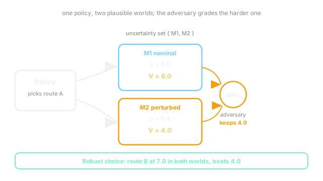
A delivery robot at state $s_0$ tries route A. Reaching the goal pays 10 and the episode ends, so $\gamma = 0$ and value equals success probability times 10. The uncertainty set holds two models:

M1 nominal: success probability $p = 0.8$ . Value is $0.8 \times 10 = 8.0$ .
M2 perturbed: a slick floor cuts success to $p = 0.4$ . Value is $0.4 \times 10 = 4.0$ .

The robust value of route A is the worse of the two: $\min(8.0, 4.0) = 4.0$ .

Now consider route B, a slower covered path with $p = 0.7$ under both models. Its value is $0.7 \times 10 = 7.0$ either way, so its robust value is $7.0$ .

Nominal planning picks A ( $8.0 > 7.0$ ). Robust planning picks B ( $7.0 > 4.0$ ). The gap between them is the price of the guarantee: $8.0 - 7.0 = 1.0$ point of nominal return traded for $3.0$ points of worst-case protection ( $7.0$ instead of $4.0$ ). This is also why robust RL differs from Q-learning, which converges to the optimal values of one fixed environment and never asks what a second environment would do.

Code

Short check of the toy above: nominal versus worst-case values, the robust pick, and its price.

1reward = 10.02
3models = {"M1 nominal": 0.8, "M2 perturbed": 0.4}4route_b_prob = 0.75
6
7def value(prob: float) -> float:8    """One-step episodic value: success probability times reward."""9    return prob * reward10
11
12for name, prob in models.items():13    print(f"{name}: V = {prob} x {reward} = {value(prob):.1f}")14
15robust_a = min(value(p) for p in models.values())16robust_b = value(route_b_prob)17print(f"Robust A = {robust_a:.1f}, Robust B = {robust_b:.1f}")18print(f"Pick B, price of safety = {value(0.8) - robust_b:.1f}")

1# -> expected output:2M1 nominal: V = 0.8 x 10.0 = 8.03M2 perturbed: V = 0.4 x 10.0 = 4.04Robust A = 4.0, Robust B = 7.05Pick B, price of safety = 1.0

Watch Out For

Playing it so safe the robot never moves

Over-pessimism is the classic failure. A huge uncertainty set makes every action look terrible, so the robust policy crawls or refuses the task entirely, even though the nominal model was right all along.

You will notice it when the price of the guarantee dwarfs the risk: giving up 1.0 point to protect 3.0 is sane, but giving up half your return to guard against a model you do not believe in is not. The fix is to shrink the set until it matches evidence, for instance a confidence region around fitted dynamics, and to report the price alongside the policy so the trade stays visible.

An uncertainty set you made up

A set with no grounding gives guarantees about nothing. Too small and the real world sits outside it, so the worst case you planned for never included the day that actually arrives. Too big and the adversary invents worlds your system will never meet, which collapses back into over-pessimism.

Fit the set from data you held out: bootstrap the dynamics, collect the models that extra environments support, and test the final policy on a left-out perturbation before you claim anything. If a new deployment breaks the policy, widen the set with that failure and re-solve.

The Quick Version

Robust RL maximizes worst-case return over an uncertainty set of models instead of expected return under one model.
The robust Bellman backup nests a $\min$ over models inside the usual $\max$ over actions, treating nature as an adversary.
In the two-route toy, route A scores 8.0 nominally but 4.0 under perturbation, while route B holds 7.0 in both worlds, so max-min picks B.
The guarantee has a price: 1.0 point of nominal return buys 3.0 points of worst-case protection here.
Rectangular, per-state uncertainty sets keep the backup tractable; correlated worst cases across states are far harder.
Calibrate the set from held-out data or the guarantee is decoration.