Sample Complexity of Exploration

Why Does This Exist?

Every exploration trick eventually faces the same awkward question: how many tries is enough? You can run epsilon-greedy for a million steps and still not know whether your policy is good or you just got lucky. Sample complexity answers that question with a number.

If you have not met these ideas yet, start here. An MDP says what the world is: states, actions, rewards, transitions, and a horizon $H$ over which returns add up. The exploration versus exploitation tradeoff says why learning hurts: you must try poorly understood actions to find out they are poor, and each try costs a real environment step. This page turns that pain into a budget: given $S$ states, $A$ actions, horizon $H$, an accuracy target $\epsilon$ (epsilon), and a failure tolerance $\delta$ (delta), how many steps before the agent can promise a near-optimal policy?

This page covers the PAC counting argument plus the RMAX and E3 intuition behind it. It does not teach the MDP itself or any specific exploration bonus; those live on the two prerequisite pages above.

Think of It Like This

How It Actually Works

PAC stands for Probably Approximately Correct. A policy $\pi$ is $\epsilon$-optimal when its value $V(\pi)$ sits within $\epsilon$ of the best achievable value $V^{\*}$, meaning $V(\pi) \ge V^{\*} - \epsilon$. The $1 - \delta$ part is the confidence: over the randomness of exploration, the promise holds with probability at least $1 - \delta$. So $(\epsilon, \delta) = (0.5, 0.05)$ reads as "within 0.5 of optimal, 95 times out of 100." Smaller $\epsilon$ means pickier. Smaller $\delta$ means surer.

Why each symbol charges you samples

$S$ (states) and $A$ (actions) set the number of things to learn: $S \times A$ state-action pairs, each needing its own visits. $H$ (horizon) stretches every estimate, because one bad transition early can corrupt a whole $H$-step return, so longer episodes demand more repeats per pair. The $1/\epsilon^2$ term is the cruel one and comes from concentration: averaging $m$ noisy samples shrinks the estimation error like $1/\sqrt{m}$, so demanding half the error needs four times the samples. The $\log(1/\delta)$ term is the bargain of the family: certainty is bought with a logarithm, so going from 95 to 99 percent confidence adds a small multiplier, not a doubling.

RMAX and E3 in one paragraph each

RMAX (Brafman and Tennenholtz, 2002) splits every pair into known or unknown. Unknown pairs get an optimistic fantasy value, the best return imaginable, which pulls the planner toward them automatically. The agent explores precisely because its model lies to it in a useful direction, and once a pair has enough visits it flips to known and the fantasy ends. E3 (Kearns and Singh, 2002) is more explicit: it runs a balanced wandering phase until its statistics say the world is known, then it freezes exploration and exploits the learned model. Both share the same moral. Exploration costs samples because unknown pairs must each be visited enough times, and optimism is just the engine that makes the agent pay up.

Worked bound instantiation

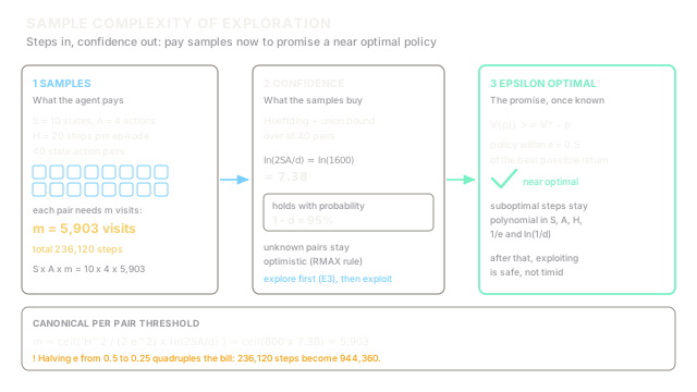
Here is one concrete instantiation so you can feel the sizes. It uses an illustrative canonical per-pair threshold in the RMAX and PAC-MDP style (Hoeffding averaging plus a union bound over all pairs, after Strehl, Li, and Littman, 2009):

$m = \left\lceil \frac{H^2}{2\epsilon^2} \ln\left(\frac{2SA}{\delta}\right) \right\rceil$

with $S = 10$ states, $A = 4$ actions, $H = 20$ steps, $\epsilon = 0.5$, and $\delta = 0.05$. Step by step:

1. Count the pairs: $S \times A = 10 \times 4 = 40$.
2. The confidence price: $\ln(2SA/\delta) = \ln(1600) \approx 7.38$.
3. The accuracy price: $H^2 / (2\epsilon^2) = 400 / 0.5 = 800$.
4. Visits per pair: $m = \lceil 800 \times 7.38 \rceil = 5{,}903$.
5. Total learning bill: $40 \times 5{,}903 = 236{,}120$ environment steps.

Now halve the accuracy target to $\epsilon = 0.25$ and everything else stays put. The accuracy price becomes $400 / 0.125 = 3{,}200$, so $m = \lceil 3{,}200 \times 7.38 \rceil = 23{,}609$ per pair and $944{,}360$ steps in total. Twice as picky, four times the bill. That is the $1/\epsilon^2$ blowup in plain numbers.

Treat the formula as a teaching shape, not a quoted theorem constant: real RMAX and PAC-MDP statements carry extra horizon factors and tighter constants depending on discounted versus finite-horizon setup. The scaling lesson survives every version: linear in $S$ and $A$, quadratic in $1/\epsilon$, logarithmic in $1/\delta$, and steep in $H$.

Code

This short script recomputes the worked example, so you can change the targets and watch the bill move.

1import math2
3
4def known_threshold(num_states, num_actions, horizon, eps, delta):5    """Illustrative canonical per-pair visit threshold (RMAX/PAC-MDP style)."""6    log_term = math.log(2 * num_states * num_actions / delta)7    return math.ceil((horizon**2 / (2 * eps**2)) * log_term)8
9
10S, A, H, EPS, DELTA = 10, 4, 20, 0.5, 0.0511m = known_threshold(S, A, H, EPS, DELTA)12print(f"log term: {math.log(2 * S * A / DELTA):.4f}")13print(f"visits per pair: {m}")14print(f"total steps: {S * A * m}")15
16m_tight = known_threshold(S, A, H, 0.25, DELTA)17print(f"halved eps per pair: {m_tight}")18print(f"halved eps total: {S * A * m_tight}")

1# -> expected output:2log term: 7.37783visits per pair: 59034total steps: 2361205halved eps per pair: 236096halved eps total: 944360

Watch Out For

The Quick Version

• Sample complexity is the number of environment steps before an agent can promise an $\epsilon$-optimal policy with probability at least $1 - \delta$.
• The bill grows with more states, more actions, and longer horizons, quadratically with $1/\epsilon$, and only logarithmically with $1/\delta$.
• RMAX explores by treating unknown pairs as optimistically wonderful, which pulls the planner toward them until visits make them known.
• E3 separates the job into two phases: wander in a balanced way until the world is known, then stop exploring and exploit the learned model.
• In the worked instantiation with 10 states, 4 actions, horizon 20, $\epsilon = 0.5$, and $\delta = 0.05$, each pair needs 5,903 visits for a total of 236,120 steps, and halving $\epsilon$ quadruples the total to 944,360.

What to Read Next

• Exploration vs. Exploitation
• Markov Decision Processes
• Temporal Difference Learning
• Q-Learning