SARSA(lambda)

Why Does This Exist?

In reinforcement learning control, an agent must discover which actions maximize cumulative reward. Standard 1-step SARSA (equivalent to $\lambda = 0$) updates only the single most recent state-action pair $(S_t, A_t)$ using the immediate transition reward and the value of the next chosen action $Q(S_{t+1}, A_{t+1})$.

While computationally simple, 1-step SARSA suffers from a severe information bottleneck:

• Glacial credit propagation: If an agent navigates a 20-step corridor to reach a $+10$ goal, 1-step SARSA only updates the final transition $(S_{19}, A_{19})$ in the first episode. The agent must successfully navigate the corridor 20 separate times for that goal reward to propagate back to the starting state $(S_0, A_0)$.
• Monte Carlo control is too volatile: Pure Monte Carlo methods update the entire trajectory at once, but they require waiting for complete episode termination, cannot learn online, and suffer from high sample variance across long, stochastic rollouts.
• $n$-step SARSA introduces latency: While $n$-step methods propagate rewards across $n$ transitions, they require maintaining explicit trajectory buffers and delay updates by $n$ steps.

SARSA($\lambda$) exists to resolve this fundamental trade-off. By extending backward-view eligibility traces from state values $V(s)$ to state-action values $Q(s, a)$, SARSA($\lambda$) gives every state-action pair an internal "memory trace" $z(s, a)$. Whenever a non-zero temporal difference error $\delta_t$ occurs, it is broadcast backward to all recently chosen actions simultaneously in real time. Credit propagates across long sequences in a single episode without storing trajectories or waiting for the episode to finish.

Think of It Like This

How It Actually Works

Action-Value Eligibility Traces and On-Policy TD Updates

Consider an environment with discrete state space $\mathcal{S}$ and action space $\mathcal{A}$. The discount factor is $\gamma \in [0, 1]$, the trace decay parameter is $\lambda \in [0, 1]$, and the step-size learning rate is $\alpha \in (0, 1]$.

1. The Action-Value Eligibility Trace Matrix

SARSA($\lambda$) maintains a short-term memory matrix $z_t \in \mathbb{R}^{|\mathcal{S}| \times |\mathcal{A}|}$ alongside its Q-table. At the start of each episode, all traces are initialized to zero:

$z_0(s, a) = 0 \quad \forall s \in \mathcal{S}, a \in \mathcal{A}$

At each time step $t$, the agent visits state $S_t$ and executes action $A_t$. The eligibility trace for $(S_t, A_t)$ can be updated using one of two strategies:

• Accumulating Traces: Increments the trace upon each visit: $z_t(s, a) = \begin{cases} \gamma \lambda z_{t-1}(s, a) + 1 & \text{if } s = S_t \text{ and } a = A_t \\ \gamma \lambda z_{t-1}(s, a) & \text{otherwise} \end{cases}$ If an agent loops repeatedly through the same state-action pair, accumulating traces can grow larger than 1, which sometimes causes value overestimation.

• Replacing Traces: Resets the trace of the chosen action to exactly 1: $z_t(s, a) = \begin{cases} 1 & \text{if } s = S_t \text{ and } a = A_t \\ 0 & \text{if } s = S_t \text{ and } a \ne A_t \\ \gamma \lambda z_{t-1}(s, a) & \text{if } s \ne S_t \end{cases}$ Replacing traces clip maximum eligibility at 1.0 and zero out competing actions in the same state, providing significantly greater stability and faster convergence in control tasks.

2. The On-Policy TD Error

After executing $A_t$ in state $S_t$, the agent receives reward $R_{t+1}$ and arrives in next state $S_{t+1}$. Crucially, the agent chooses its next action $A_{t+1}$ according to its behavior policy $\pi$ (such as $\varepsilon$-greedy with respect to current Q-values).

The temporal difference error $\delta_t$ is computed on-policy:

$\delta_t = R_{t+1} + \gamma Q_t(S_{t+1}, A_{t+1}) - Q_t(S_t, A_t)$

If $S_{t+1}$ is a terminal state, $Q_t(S_{t+1}, A_{t+1})$ is treated as 0.

3. Global Broadcast Update

Instead of updating only $(S_t, A_t)$, the scalar error $\delta_t$ updates every state-action pair simultaneously, scaled by its eligibility trace:

$Q_{t+1}(s, a) = Q_t(s, a) + \alpha \delta_t z_t(s, a) \quad \forall s \in \mathcal{S}, a \in \mathcal{A}$

Finally, all traces decay by factor $\gamma \lambda$ in preparation for the next time step:

$z_{t+1}(s, a) = \gamma \lambda z_t(s, a) \quad \forall s \in \mathcal{S}, a \in \mathcal{A}$

Notice the spectrum of $\lambda$:

• When $\lambda = 0$: Only the current pair has $z(S_t, A_t) = 1$ while all past traces immediately decay to 0, reducing the algorithm exactly to standard 1-step SARSA.
• When $\lambda = 1$: Traces decay strictly by the discount factor $\gamma$, causing updates to approximate online Monte Carlo control.
• When $0 < \lambda < 1$: The agent achieves the optimal trade-off between fast credit assignment and low variance.

Worked numerical example

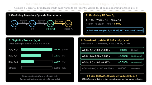
Let us trace a 3-step navigation sequence through a discrete grid world to see how SARSA($\lambda$) rewards past actions in a single episode:

$\text{Trajectory: } (S_0, \text{right}) \xrightarrow{R_1 = 0.0} (S_1, \text{up}) \xrightarrow{R_2 = 0.0} (S_2, \text{right}) \xrightarrow{R_3 = 10.0} (S_3, \text{Terminal})$

Parameters:

• Discount factor $\gamma = 0.9$
• Trace decay $\lambda = 0.7 \implies \gamma \lambda = 0.9 \times 0.7 = 0.6300$
• Learning rate $\alpha = 0.1$
• Replacing traces
• Initial $Q(s, a) = 0.0$ and $z(s, a) = 0.0$ for all pairs

Step 0 ($t=0$): Transition $(S_0, \text{right}) \to (S_1, \text{up})$ with $R_1 = 0.0$

1. Trace update: $z(S_0, \text{right}) = 1.0000, \quad \text{all other } z = 0.0$
2. TD error: $\delta_0 = R_1 + \gamma Q(S_1, \text{up}) - Q(S_0, \text{right}) = 0.0 + 0.9(0.0) - 0.0 = 0.0000$
3. Q update: $\delta_0 = 0 \implies Q(s, a)$ remains $0.0$.
4. Trace decay: $z(S_0, \text{right}) \leftarrow 0.63 \times 1.0000 = 0.6300$

Step 1 ($t=1$): Transition $(S_1, \text{up}) \to (S_2, \text{right})$ with $R_2 = 0.0$

1. Trace update: $z(S_1, \text{up}) = 1.0000, \quad z(S_0, \text{right}) = 0.6300$
2. TD error: $\delta_1 = R_2 + \gamma Q(S_2, \text{right}) - Q(S_1, \text{up}) = 0.0 + 0.9(0.0) - 0.0 = 0.0000$
3. Q update: $\delta_1 = 0 \implies Q(s, a)$ remains $0.0$.
4. Trace decay: $z(S_1, \text{up}) \leftarrow 0.63 \times 1.0000 = 0.6300$ $z(S_0, \text{right}) \leftarrow 0.63 \times 0.6300 = 0.3969$

Step 2 ($t=2$): Transition $(S_2, \text{right}) \to S_3$ with $R_3 = 10.0$ (Goal Reached)

1. Trace update: $z(S_2, \text{right}) = 1.0000, \quad z(S_1, \text{up}) = 0.6300, \quad z(S_0, \text{right}) = 0.3969$
2. On-policy TD error (Terminal, so $Q(S_3) = 0$): $\delta_2 = R_3 + \gamma(0.0) - Q(S_2, \text{right}) = 10.0 + 0.0 - 0.0 = \mathbf{+10.0000}$
3. Global broadcast update ($\alpha \delta_2 = 0.1 \times 10.0 = 1.0000$):
   • For $(S_2, \text{right})$: $Q(S_2, \text{right}) \leftarrow 0.0 + 1.0000 \times 1.0000 = \mathbf{+1.0000}$
   • For $(S_1, \text{up})$: $Q(S_1, \text{up}) \leftarrow 0.0 + 1.0000 \times 0.6300 = \mathbf{+0.6300}$
   • For $(S_0, \text{right})$: $Q(S_0, \text{right}) \leftarrow 0.0 + 1.0000 \times 0.3969 = \mathbf{+0.3969}$
   • For all unvisited pairs: $Q(s, a) \leftarrow 0.0 + 1.0000 \times 0.0000 = \mathbf{0.0000}$

Comparison with 1-Step SARSA

In standard 1-step SARSA, neither $(S_1, \text{up})$ nor $(S_0, \text{right})$ learned anything from this goal. In SARSA($\lambda$), both actions immediately acquired positive value estimates in that very same episode.

Code

The following self-contained Python implementation trains a tabular SARSA($\lambda$) agent on a linear navigation grid, demonstrating eligibility trace accumulation, on-policy error broadcasting, and automated assertions.

1from typing import Dict, List, Tuple2
3
4class MiniGridSARSA:5    """Tabular SARSA(lambda) control on a discrete linear gridworld.6
7    Layout: S0 <-> S1 <-> S2 <-> S3 (Terminal Goal, Reward = +10.0)8    Actions: 0 = 'left', 1 = 'right'9    """10
11    def __init__(12        self,13        num_states: int = 4,14        gamma: float = 0.9,15        lam: float = 0.7,16        alpha: float = 0.1,17        trace_type: str = "replacing",18    ) -> None:19        self.num_states = num_states20        self.goal_state = num_states - 121        self.actions = [0, 1]  # 0: left, 1: right22        self.gamma = gamma23        self.lam = lam24        self.alpha = alpha25        self.trace_type = trace_type26
27        # Initialize Q-table and eligibility trace matrix to 0.028        self.q_table: Dict[Tuple[int, int], float] = {29            (s, a): 0.0 for s in range(num_states) for a in self.actions30        }31        self.z_traces: Dict[Tuple[int, int], float] = {32            (s, a): 0.0 for s in range(num_states) for a in self.actions33        }34
35    def choose_action(self, state: int) -> int:36        """Deterministic policy that prefers 'right' (1) on value ties."""37        q_left = self.q_table[(state, 0)]38        q_right = self.q_table[(state, 1)]39        return 1 if q_right >= q_left else 040
41    def step_environment(42        self, state: int, action: int43    ) -> Tuple[int, float, bool]:44        """Executes action in environment. Moving right advances state."""45        if action == 1:46            next_state = min(state + 1, self.goal_state)47        else:48            next_state = max(state - 1, 0)49
50        done = next_state == self.goal_state51        reward = 10.0 if done else 0.052        return next_state, reward, done53
54    def train_episode(self) -> int:55        """Executes a single on-policy episode of SARSA(lambda)."""56        # Traces must be zeroed out at the start of every episode57        for key in self.z_traces:58            self.z_traces[key] = 0.059
60        state = 061        action = self.choose_action(state)62        step_count = 063
64        while state != self.goal_state and step_count < 50:65            next_state, reward, done = self.step_environment(state, action)66            next_action = self.choose_action(next_state) if not done else 067
68            # 1. Update eligibility trace for current state-action pair69            if self.trace_type == "replacing":70                # Replacing trace: set chosen action to 1.0, other actions in state to 0.071                for a in self.actions:72                    self.z_traces[(state, a)] = 1.0 if a == action else 0.073            else:74                # Accumulating trace: add 1.0 to visited pair75                self.z_traces[(state, action)] += 1.076
77            # 2. Compute on-policy TD error delta_t78            q_next = (79                self.q_table[(next_state, next_action)] if not done else 0.080            )81            td_error = (82                reward + self.gamma * q_next - self.q_table[(state, action)]83            )84
85            # 3. Global broadcast update across all state-action pairs86            for pair in self.q_table:87                self.q_table[pair] += (88                    self.alpha * td_error * self.z_traces[pair]89                )90                # 4. Decay traces by gamma * lambda91                self.z_traces[pair] *= self.gamma * self.lam92
93            state = next_state94            action = next_action95            step_count += 196
97        return step_count98
99
100# Instantiate and train agent on episode 1101agent = MiniGridSARSA(102    num_states=4, gamma=0.9, lam=0.7, alpha=0.1, trace_type="replacing"103)104steps_taken = agent.train_episode()105
106print(f"Episode completed in {steps_taken} steps.")107print(f"Q(S0, right): {agent.q_table[(0, 1)]:.4f}")108print(f"Q(S1, right): {agent.q_table[(1, 1)]:.4f}")109print(f"Q(S2, right): {agent.q_table[(2, 1)]:.4f}")110
111# Validate multi-step credit assignment with assertions112assert steps_taken == 3, f"Expected 3 steps, got {steps_taken}"113assert round(agent.q_table[(2, 1)], 4) == 1.0000, "S2 Q-value incorrect"114assert round(agent.q_table[(1, 1)], 4) == 0.6300, "S1 Q-value incorrect"115assert round(agent.q_table[(0, 1)], 4) == 0.3969, "S0 Q-value incorrect"116print("Assertions passed: Multi-step credit propagated in a single episode!")117
118# -> Expected output:119# -> Episode completed in 3 steps.120# -> Q(S0, right): 0.3969121# -> Q(S1, right): 0.6300122# -> Q(S2, right): 1.0000123# -> Assertions passed: Multi-step credit propagated in a single episode!

Watch Out For

The Quick Version

• Action-value traces: SARSA($\lambda$) extends eligibility traces from states $V(s)$ to state-action pairs $Q(s, a)$ by maintaining a trace matrix $z(s, a) \in \mathbb{R}^{|\mathcal{S}| \times |\mathcal{A}|}$.
• Backward broadcast: Whenever an on-policy transition produces a TD error $\delta_t$, that single error updates all recently visited $(s, a)$ pairs simultaneously, weighted by $z(s, a)$.
• Single-episode propagation: Downstream rewards propagate backward across multi-step trajectories in a single episode, eliminating the one-step propagation bottleneck of standard SARSA.
• Strictly on-policy: The target evaluates $Q(S_{t+1}, A_{t+1})$ using the action actually selected by the exploratory policy, preserving convergence guarantees without complex trace-cutting logic.

What to Read Next

• Backward View of TD(lambda)
• Watkins's Q(lambda)
• Q-Learning vs SARSA