Watkins's Q(lambda)
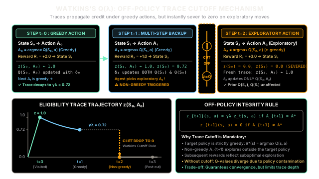
Watkins's Q(lambda) extends eligibility traces to off-policy Q-learning, propagating reward signals backward across multi-step action trajectories. To maintain target policy validity, it immediately zeroes all eligibility traces whenever the agent executes an exploratory, non-greedy action.
Why Does This Exist?
In reinforcement learning, standard Q-learning is a landmark algorithm because it is off-policy: it learns the optimal action-value function while following an arbitrary, exploratory behavior policy such as -greedy. However, classical Q-learning performs only one-step updates:
Because information propagates back only one state-action transition per time step, credit assignment is painfully slow. If an agent navigates a 100-step gridworld before reaching a terminal goal reward, standard Q-learning requires at least 100 separate episodes for that reward signal to trickle all the way back to the initial start state.
In on-policy methods, SARSA() overcomes this bottleneck using eligibility traces, allowing an immediate TD error to update all previously visited state-action pairs simultaneously. But naively applying eligibility traces to Q-learning creates a fundamental mathematical contradiction:
- The target policy being learned in Q-learning is the strictly greedy policy .
- The behavior policy generating the agent's actions is exploratory (e.g., selecting random exploratory actions with probability ).
- If an agent selects an exploratory action , all subsequent rewards from step onward are generated by a suboptimal, exploratory trajectory. Crediting earlier state-action pairs with rewards generated by exploratory deviations violates the Bellman optimality equation and biases action-value estimates.
In 1989, Christopher Watkins solved this theoretical dilemma by introducing Watkins's . The algorithm maintains eligibility traces to accelerate multi-step credit assignment, but enforces a strict cutoff rule: eligibility traces accumulate and decay smoothly as long as the agent selects greedy actions, but the instant the agent selects an exploratory, non-greedy action, all eligibility traces are immediately reset to zero.
Think of It Like This
A High-Speed Train Navigating Track Switches
Imagine a high-speed express train traveling down a mainline rail corridor between cities:
- Riding the Express Line (Greedy Actions): As long as every track switch aligns with the optimal express corridor (), the train maintains high velocity and smooth momentum. Any progress signal or clearance milestone (a reward) can be credited back to the entire sequence of track segments just passed. The train's historical momentum log—its eligibility trace—decays smoothly by , carrying multi-step credit backward.
- Taking an Exploratory Siding Switch (Non-Greedy Action): Suppose the conductor decides to test an unknown siding switch just to see where it leads (an exploratory move under -greedy). The train branches off onto a slow, unpaved industrial siding.
- The Immediate Momentum Reset: You cannot evaluate the speed of the mainline express route using the bumpy delays encountered on the industrial spur! The mainline momentum is instantly broken. The conductor must hit the reset button on the express route log: all historical momentum traces are severed to zero.
- Resuming the Journey: The train evaluates the single immediate transition onto the siding, and then begins building fresh traces from that point forward. The historical mainline segments are protected from being falsely blamed or credited for whatever happens down the exploratory detour.
Where the analogy breaks down: A physical train with mass cannot instantly drop kinetic momentum to zero without a catastrophic derailment. In algorithmic reinforcement learning, eligibility traces are mathematical memory buffers stored in RAM that can be reset to zero in time without physical consequence. Furthermore, an agent can return to the optimal greedy track on the very next time step and resume multi-step trace accumulation immediately.
How It Actually Works
Off-Policy Learning Meets Eligibility Traces
Watkins's tracks two data structures across all state-action pairs :
- The action-value estimate matrix .
- The eligibility trace matrix , initialized to zero.
At each time step , the agent visits state , takes action , observes reward , and transitions to state . The algorithm proceeds through five structured operations:
1. Compute the Greedy Action and TD Error
The algorithm computes the optimal greedy action in the next state :
The TD error is computed using the greedy evaluation, exactly as in classical Q-learning:
where is the discount factor.
2. Increment the Eligibility Trace
The trace for the current state-action pair is incremented. Under accumulating traces:
Under replacing traces (which often yields superior empirical stability):
3. Update Action-Values Across All Active Traces
Every state-action pair in the state space is updated proportional to its current trace:
where is the step-size learning rate.
4. The Watkins Trace Cutoff Rule
Before transitioning to step , the agent selects its next action using its behavior policy (such as -greedy). The eligibility traces are then updated for the subsequent step according to the Watkins Cutoff Rule:
where is the trace decay parameter.
Why the Cutoff is Mandatory
To understand why traces must zero out, consider the theoretical multi-step return target:
This -step return is a valid estimate of the optimal action-value only if all intermediate actions were chosen according to the optimal target policy .
If the behavior policy selects an exploratory action at step (), the subsequent reward reflects that exploratory action rather than the optimal policy. Permitting eligibility traces to survive beyond step would backpropagate into , contaminating the optimal value estimate with exploratory noise. Setting truncates the multi-step return at the point of exploratory divergence, preserving the mathematical integrity of the Bellman optimality operator.
Worked numerical example
Let us trace Watkins's through a concrete 3-step sequence:
System Parameters
- Discount factor:
- Trace decay parameter: (giving product )
- Learning rate:
- Actions:
Initial Values
All initial eligibility traces .
Step 0 (): Greedy Move
- Action & Transition: Agent at takes . Receives reward and enters .
- Trace Increment: .
- Target Evaluation: At , (achieved by ).
- TD Error:
- Q-Value Update:
- Next Action Selected: Agent selects for state . Because , the trace survives and decays:
Step 1 (): Multi-Step Credit & Trace Severing
- Action & Transition: Agent at takes . Receives reward and enters .
- Trace Increment: . Notice is still active.
- Target Evaluation: At , (achieved by ).
- TD Error:
- Multi-Step Value Updates:
- For :
- For (multi-step credit propagates backward!):
- Next Action Selected: Agent's behavior policy selects an exploratory action: . Because (since ), the Watkins Cutoff Rule triggers: All eligibility traces across the entire state space are severed to zero.
Step 2 (): Post-Cutoff Exploration
- Action & Transition: Agent at executes exploratory action . Receives reward and reaches terminal state .
- Trace Increment: . Prior traces remain zero: , .
- Target Evaluation: Terminal state has .
- TD Error:
- Value Updates:
- For :
- For : Trace is , so remains (completely untouched).
- For : Trace is , so remains (completely untouched).
The exploratory reward was safely quarantined to without contaminating earlier optimal policy evaluations.
Code
The following self-contained, type-hinted Python script implements Watkins's and includes explicit assertions confirming trace preservation under greedy actions and complete trace zeroing under exploratory actions:
from typing import Dict, List, Tuple
class WatkinsQLambda: """Watkins's Q(lambda) off-policy control algorithm with eligibility traces."""
def __init__( self, states: List[str], actions: List[str], alpha: float = 0.2, gamma: float = 0.9, lam: float = 0.8, replacing_traces: bool = False, ) -> None: self.states = states self.actions = actions self.alpha = alpha self.gamma = gamma self.lam = lam self.replacing_traces = replacing_traces
# Initialize Q-table and eligibility trace table to zero self.q: Dict[Tuple[str, str], float] = { (s, a): 0.0 for s in states for a in actions } self.z: Dict[Tuple[str, str], float] = { (s, a): 0.0 for s in states for a in actions }
def get_greedy_action(self, state: str) -> str: """Return the optimal greedy action for a given state.""" q_vals = {a: self.q[(state, a)] for a in self.actions} max_v = max(q_vals.values()) return [a for a in self.actions if q_vals[a] == max_v][0]
def step_update( self, state: str, action: str, reward: float, next_state: str, next_action: str, is_terminal: bool, ) -> Tuple[float, bool]: """Perform a Watkins's Q(lambda) update step.
Returns: Tuple of (TD error delta, boolean indicating whether next action is greedy). """ # 1. Evaluate greedy action in next state if is_terminal: max_q_next = 0.0 next_action_is_greedy = True else: best_action = self.get_greedy_action(next_state) max_q_next = self.q[(next_state, best_action)] next_action_is_greedy = (next_action == best_action)
# 2. Compute Q-learning TD error: delta = R + gamma * max_a Q(S', a) - Q(S, A) delta = reward + self.gamma * max_q_next - self.q[(state, action)]
# 3. Increment eligibility trace for the current state-action pair if self.replacing_traces: self.z[(state, action)] = 1.0 else: self.z[(state, action)] += 1.0
# 4. Multi-step value update across all active traces for s in self.states: for a in self.actions: self.q[(s, a)] += self.alpha * delta * self.z[(s, a)]
# 5. Watkins trace update / cutoff rule for subsequent step if next_action_is_greedy: # Greedy action: traces survive and decay exponentially for s in self.states: for a in self.actions: self.z[(s, a)] *= self.gamma * self.lam else: # Exploratory action: sever all eligibility traces to zero for s in self.states: for a in self.actions: self.z[(s, a)] = 0.0
return delta, next_action_is_greedy
def demonstrate_watkins_q_lambda() -> None: states = ["S0", "S1", "S2", "S3"] actions = ["greedy", "exploratory"] agent = WatkinsQLambda( states, actions, alpha=0.2, gamma=0.9, lam=0.8, replacing_traces=False )
# Initialize Q-values matching the worked numerical example agent.q[("S0", "greedy")] = 4.0 agent.q[("S0", "exploratory")] = 2.0 agent.q[("S1", "greedy")] = 5.0 agent.q[("S1", "exploratory")] = 3.0 agent.q[("S2", "greedy")] = 6.0 agent.q[("S2", "exploratory")] = 1.0
print("--- Step 0: Greedy Action (Trace Survives & Decays) ---") d0, is_g0 = agent.step_update("S0", "greedy", 2.0, "S1", "greedy", False) print(f"delta_0: {d0:.4f}") print(f"Q(S0, greedy): {agent.q[('S0', 'greedy')]:.4f}") print(f"z(S0, greedy) after decay: {agent.z[('S0', 'greedy')]:.4f}") assert abs(agent.z[("S0", "greedy")] - 0.72) < 1e-6 assert is_g0 is True
print("\n--- Step 1: Multi-Step Backup, followed by Exploratory Selection ---") d1, is_g1 = agent.step_update("S1", "greedy", 1.0, "S2", "exploratory", False) print(f"delta_1: {d1:.4f}") print(f"Q(S0, greedy): {agent.q[('S0', 'greedy')]:.4f} (multi-step credit applied!)") print(f"Q(S1, greedy): {agent.q[('S1', 'greedy')]:.4f}") print(f"Next action greedy? {is_g1}") print(f"z(S0, greedy) after cutoff: {agent.z[('S0', 'greedy')]:.4f}") print(f"z(S1, greedy) after cutoff: {agent.z[('S1', 'greedy')]:.4f}")
# Explicitly assert that all traces are strictly zeroed out for s in states: for a in actions: assert agent.z[(s, a)] == 0.0, f"Trace not zeroed at ({s}, {a})!"
print("\n--- Step 2: Exploratory Action (Severed Credit Horizon) ---") d2, is_g2 = agent.step_update("S2", "exploratory", 3.0, "S3", "greedy", True) print(f"delta_2: {d2:.4f}") print(f"Q(S0, greedy): {agent.q[('S0', 'greedy')]:.4f} (UNTOUCHED by exploratory reward)") print(f"Q(S1, greedy): {agent.q[('S1', 'greedy')]:.4f} (UNTOUCHED by exploratory reward)") print(f"Q(S2, exploratory): {agent.q[('S2', 'exploratory')]:.4f}")
assert abs(agent.q[("S0", "greedy")] - 4.7016) < 1e-4 assert abs(agent.q[("S1", "greedy")] - 5.2800) < 1e-4 assert abs(agent.q[("S2", "exploratory")] - 1.4000) < 1e-4
if __name__ == "__main__": demonstrate_watkins_q_lambda()
# -> Expected output:# -> --- Step 0: Greedy Action (Trace Survives & Decays) ---# -> delta_0: 2.5000# -> Q(S0, greedy): 4.5000# -> z(S0, greedy) after decay: 0.7200# -> # -> --- Step 1: Multi-Step Backup, followed by Exploratory Selection ---# -> delta_1: 1.4000# -> Q(S0, greedy): 4.7016 (multi-step credit applied!)# -> Q(S1, greedy): 5.2800# -> Next action greedy? False# -> z(S0, greedy) after cutoff: 0.0000# -> z(S1, greedy) after cutoff: 0.0000# -> # -> --- Step 2: Exploratory Action (Severed Credit Horizon) ---# -> delta_2: 2.0000# -> Q(S0, greedy): 4.7016 (UNTOUCHED by exploratory reward)# -> Q(S1, greedy): 5.2800 (UNTOUCHED by exploratory reward)# -> Q(S2, exploratory): 1.4000Watch Out For
The Trace Contamination Trap: Failing to Zero Traces on Exploratory Actions
A frequent bug when transitioning from on-policy SARSA() to off-policy Q-learning is blindly retaining standard exponential trace decay () without checking whether the next action was greedy.
The Symptom: If eligibility traces are allowed to persist across exploratory transitions:
- Severe Value Pollution: Earlier optimal decisions receive credit or blame for random exploratory actions taken downstream. If an exploratory action falls off a cliff, the entire prior trajectory of high-quality decisions is erroneously penalized.
- Convergence Failure: The algorithm no longer optimizes the Bellman optimality equation. Instead, it converges toward the value function of a corrupted hybrid policy, producing suboptimal control decisions.
- Instability in Large State Spaces: In environments with function approximation, trace contamination triggers unbounded value oscillations and gradient instability.
The Fix:
- Always inspect the chosen behavioral action against the greedy action set . If is not in the greedy set, execute a hard reset:
z.fill(0.0). - Be mindful of the trace death penalty: in highly exploratory regimes (e.g., ), traces are cut on average every 5 steps, reducing Watkins's to 1-step Q-learning. If long multi-step off-policy traces are essential in your domain, use modern algorithms like Tree Backup() or Retrace(), which scale trace decay continuously by the target policy probability rather than abruptly killing the entire trace.
The Quick Version
- Accelerated Off-Policy Learning: Watkins's bridges multi-step eligibility traces with off-policy Q-learning, enabling rapid credit assignment without waiting for full episodes to terminate.
- The Cutoff Invariant: Traces decay smoothly by as long as the agent selects greedy actions; the moment an exploratory non-greedy action is chosen, all traces across the entire state space are set strictly to zero.
- Preserving Bellman Optimality: Zeroing traces is mathematically required because downstream rewards generated after an exploratory deviation cannot be used to evaluate the optimal target policy .
- The Exploration Trade-Off: While Watkins's cutoff guarantees unbiased convergence, high behavioral exploration rates frequently sever traces, causing the algorithm's effective lookahead horizon to collapse back toward 1-step Q-learning.