Sim-to-Real Transfer

Train a robot brain across thousands of fake physics settings in simulation, then ship that same brain to the real robot with no extra training, as long as reality falls inside the range you trained on.

Why Does This Exist?

Real practice is slow, pricey, and sometimes dangerous. A walking robot that needs a million falls to learn will shred its gears long before it gets good, and every one of those falls costs a real hour. Simulation flips the economics: you can run thousands of fake robots in parallel and collect years of falls in an afternoon, for the price of electricity.

The catch is the reality gap: no simulator copies physics exactly. Friction, mass, motor lag, and sensor noise all differ a little, and a policy trained on one exact fake world often collapses on the real one. That gap is why sim-to-real transfer exists as its own skill.

Two basics before we go on. A policy is the rule the agent follows: given the current state, which action to take. An MDP is the math frame around it: states, actions, and transition dynamics that say what happens next. If either term feels shaky, read model-based RL for dynamics and planning, and deep reinforcement learning for how neural nets represent policies from raw sensors.

Scope note: the embodiment overview lives on the simulation page, which is about why robots train in fake worlds at all. This page is the RL transfer method: the three ways across the gap, a hand-worked friction and mass example, and the checklist for shipping with no extra training.

Think of It Like This

The Cook Who Trained in Every Kitchen

Suppose you want a cook who can walk into any stranger's kitchen and nail dinner on the first try, no practice round.

The one-kitchen cook trains for a year on the same gas stove. They learn exactly when that burner sears. Put them on an electric coil and dinner burns, because every habit is tuned to one stove.
The every-kitchen cook trains across gas, electric, and induction, at sea level and up a mountain, with thin pans and heavy ones. Each week the kitchen changes. They stop trusting exact burner timings and start watching the food: sizzle sound, color, smell. Those cues survive every kitchen.
Test day is a kitchen they have never seen. It still works, because the new stove sits somewhere inside the range they already survived. No practice round needed.

The mapping: kitchens are simulators with different physics settings, the cook's habits are the policy, watching the food instead of the clock is learning feedback cues that survive the gap, and the unseen kitchen is the real robot.

Where the analogy stops: you can see a stove is electric before you cook. A robot cannot see its true friction or mass; it must act well across all of them at once. And kitchens differ in a few obvious ways, while physics settings drift continuously and interact, so covering the range takes deliberate sampling, not just variety for its own sake.

How It Actually Works

The gap, stated plainly

Write the simulator's dynamics as $P_{sim}(s' \mid s, a)$ : the probability of landing in next state $s'$ after taking action $a$ in state $s$ . The real world's dynamics are $P_{real}(s' \mid s, a)$ , same shape, slightly different numbers. The reality gap is the mismatch between those two. A policy $\pi(a \mid s)$ trained to be brilliant under $P_{sim}$ can fail under $P_{real}$ because it leaned on details that were only true in the fake world, like one exact friction value.

Three families of fixes exist, and they stack:

Domain randomization widens the simulator. Each episode samples fresh physics settings, like friction $\mu$ (a unitless grip number, higher means grippier) and mass $m$ in kilograms, from a range you choose. The policy must earn reward across all of them, so it stops trusting any single one.
System identification narrows the simulator. You measure the real robot (weigh the links, slide a test block to estimate friction) and set the simulator to match. This shrinks the gap directly but never to zero, because some things, like cable stiffness, resist measuring.
Adaptation keeps learning after shipping. The deployed policy gets a small number of real trials, or an adapter module reads recent history and adjusts. This rescues transfers that just miss, at the cost of real-world trials you hoped to skip.

Randomization is the default when real trials are expensive, identification pays when a parameter dominates the task, and adaptation is the safety net when neither quite closes the gap.

Worked example: friction and mass ranges

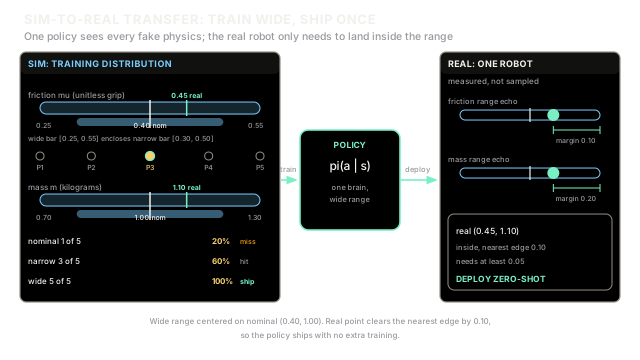
Take a block-pushing task. Success means the block stops inside a target zone. The two physics settings that matter are friction $\mu$ and block mass $m$ in kilograms. The nominal simulator both developers started from uses $\mu_0 = 0.40$ and $m_0 = 1.00$ .

Three policies, three training setups:

Nominal-only trains at the single point $\mu = 0.40$ , $m = 1.00$ .
Narrow samples $\mu$ uniformly from $[0.30, 0.50]$ and $m$ uniformly from $[0.80, 1.20]$ . Width check: $0.50 - 0.30 = 0.20$ for friction, $1.20 - 0.80 = 0.40$ for mass.
Wide samples $\mu$ uniformly from $[0.25, 0.55]$ and $m$ uniformly from $[0.70, 1.30]$ . Width check: $0.55 - 0.25 = 0.30$ for friction, $1.30 - 0.70 = 0.60$ for mass. Center check: $(0.25 + 0.55) / 2 = 0.40$ and $(0.70 + 1.30) / 2 = 1.00$ , so the wide range is centered on the same nominal point.

Now grade all three on five fixed probe settings that span the wide range, using one stated pass rule: a probe passes if it sits inside the policy's training rectangle, boundaries included. This rule is a simplification that stands in for full rollouts; it isolates what range width alone buys.

Probe P1 at $(\mu = 0.25, m = 0.70)$ : nominal misses, narrow misses, wide hits.
Probe P2 at $(\mu = 0.32, m = 0.85)$ : nominal misses, narrow hits ( $0.32$ and $0.85$ both inside), wide hits.
Probe P3 at $(\mu = 0.40, m = 1.00)$ : all three hit.
Probe P4 at $(\mu = 0.48, m = 1.15)$ : nominal misses, narrow hits, wide hits.
Probe P5 at $(\mu = 0.55, m = 1.30)$ : nominal misses, narrow misses, wide hits on the boundary.

Count the passes:

Nominal-only passes 1 of 5, which is $1 / 5 = 0.20$ or 20 percent.
Narrow passes 3 of 5, which is $3 / 5 = 0.60$ or 60 percent.
Wide passes 5 of 5, which is $5 / 5 = 1.00$ or 100 percent.

The real robot measures in at $\mu_{real} = 0.45$ and $m_{real} = 1.10$ . Nominal-only misses it. Narrow covers it. Wide covers it with room to spare: friction margins are $0.45 - 0.25 = 0.20$ below and $0.55 - 0.45 = 0.10$ above, mass margins are $1.10 - 0.70 = 0.40$ below and $1.30 - 1.10 = 0.20$ above, so the nearest edge is $0.10$ away in friction.

The zero-shot deploy checklist

Zero-shot means the shipped policy gets no real-world practice trials. Ship it when all three hold:

The real setting sits inside the training range on every randomized axis, with margin. Our rule of thumb: at least $0.05$ of clearance to the nearest edge, and the worked transfer clears it at $0.10$ .
Simulated success stays flat, not spiky, across the range. If the edges of your range score far worse than the center, widen testing there before trusting the middle.
Nothing load-bearing was left out of the randomization. Cameras, delays, and sensor noise count as settings too; a dynamics-only range plus a new camera is a transfer you have not tested.

Watch Out For

Randomizing so wide the policy learns nothing

The symptom: training reward climbs, then stalls far below the nominal-only score, and the robot moves like it is afraid of its own shadow. That happens when the range includes settings no real robot will ever meet, like frictionless ice next to glue, and the policy spends its capacity surviving fantasies instead of solving your room.

The fix: cap each axis at plausible hardware plus a stated margin, then grow only the axis whose probes fail. Our worked example grows friction from width $0.20$ to $0.30$ because probes P1 and P5 failed, not because wider is always better.

An unmodeled effect eats the transfer

The symptom: sim probes pass at 100 percent and the real robot still fails on day one. The usual culprits are effects the simulator never varied: camera exposure, control delay, gear backlash, or a flexing mount. Your margin math only covers axes you randomized.

The fix: before shipping, list every sensor and timing path between the policy and the motors, and either randomize it or measure it. If the camera changed since training, that is a new transfer, and no friction margin covers it.

The Quick Version

Sim-to-real transfer exists because real practice is slow and breakable while simulation is cheap, and the two disagree on physics details called the reality gap.
Domain randomization trains one policy across a range of physics settings so it stops trusting any single fake value.
System identification measures the real robot to shrink the gap, and adaptation spends a few real trials to mop up what is left.
In the worked example, widening friction from width 0.20 to 0.30 and mass from 0.40 to 0.60 lifts probe success from 3 of 5 to 5 of 5.
Ship zero-shot only when the real robot lands inside the trained range with margin on every axis, sim success is flat across the range, and no sensor or delay was left out.