Model-Based Reinforcement Learning

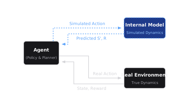
A model based agent learns a simulator of its world, then practices inside that simulator thousands of times before spending one real action.

A 2 step imagined rollout from position 2.0 predicts 2.8 then 3.5 with rewards 1.0 and 1.0, giving a planned return of 1.9 before any real move

Why Does This Exist?

Trial and error in the real world is slow, costly, and sometimes unsafe. A robot arm learning to grip by dropping fragile objects, or a chemical controller learning by overshooting pressure limits, pays for every lesson in damage. Model free agents accept that bill: they update only from real transitions $(s, a, r, s')$ .

Model based RL buys a way out. The agent first learns how the world responds, an approximation $\hat{p}(s' \mid s, a)$ of the transition dynamics plus a reward model $\hat{r}(s, a)$ , then plans inside that simulator. Thousands of imagined trajectories cost milliseconds and break nothing. The catch is that the simulator is always slightly wrong, so the agent must keep checking its plans against fresh real experience. This page teaches that loop of learning the model, planning in it, and re grounding in reality. The decision process underneath is in MDP foundations, the classic architecture that mixes real and imagined updates is Dyna, and the deep learning version is model-based deep RL.

The one idea you need first

An MDP is the tuple $(\mathcal{S}, \mathcal{A}, p, r, \gamma)$ : states, actions, true transition probabilities $p$ , rewards $r$ , and discount $\gamma$ . A model based agent never sees $p$ and $r$ directly. It collects real transitions and fits approximations $\hat{p}$ and $\hat{r}$ with supervised learning, then treats those approximations as a simulator.

Think of It Like This

A chess player who learned the rules, then thinks ahead

A beginner who never learned how the pieces move can only learn by playing full games and remembering which moves lost material. Every lesson costs a finished game.

Once you know the rules, you change strategy. You look at the board, picture knight takes pawn three moves out, picture the reply, and pick the line with the best outcome, all before touching a piece. You still play real games, because your mental board misses things, but each real game now teaches your mental model instead of just one move.

That is the split: the rules are the learned model, the picturing is planning, and the real games are the grounding steps. Where it stops: chess rules are exact, while a learned dynamics model is approximate, so the agent must quantify uncertainty and replan far more often than a chess player rearranges pieces.

How It Actually Works

1. Learning the model from real transitions

The agent acts in the real environment and stores $(s_t, a_t, r_t, s_{t+1})$ tuples. It fits a transition model $\hat{s}_{t+1} \approx \hat{p}(s_t, a_t)$ and a reward model $\hat{r}_t \approx \hat{r}(s_t, a_t)$ . In a grid world this can be counts in a table. In continuous control it is usually a neural network trained to minimize prediction error on those tuples.

2. Planning inside the model

With the simulator in hand, the agent searches imagined futures without touching the world. Two common styles are trajectory rollouts, where many action sequences are simulated and the first action of the best one is executed, and background planning in the Dyna style, where stored states are resampled, stepped through the model, and used for value updates exactly as if they were real.

3. Acting, observing, and updating the model

Because $\hat{p}$ is never perfect, the loop must close: act with the current plan, observe the true $s'$ and $r$ , retrain the model on the new tuple, and replan. Planning gains speed. Grounding keeps the plans honest.

Worked example

Track a cart on a line with discount $\gamma = 0.9$ . The learned model predicts position updates and rewards:

Start at real position $s_0 = 2.0$ and consider pushing right twice, $a_0 = +1$ then $a_1 = +1$ . The model predicts $\hat{s}_1 = 2.8$ with $\hat{r}_0 = 1.0$ , then from there $\hat{s}_2 = 3.5$ with $\hat{r}_1 = 1.0$ . The planned return is

\hat{G}_0 = \hat{r}_0 + \gamma \hat{r}_1 = 1.0 + 0.9 \times 1.0 = 1.0 + 0.9 = 1.9

The agent compares this 1.9 against the imagined returns of pushing left or standing still, executes the first action of the best sequence in the real world, and uses the true outcome to improve the model. No real steps were spent evaluating the losing sequences.

Code

This snippet replays the worked example: it steps the tiny learned model twice from 2.0 and prints the planned return, which must read 1.9.

1def learned_model(state: float, action: float) -> tuple[float, float]:2    deltas = {(2.0, 1.0): (0.8, 1.0), (2.8, 1.0): (0.7, 1.0)}3    return deltas.get((round(state, 1), action), (0.0, 0.0))4
5
6def planned_return(start: float, actions: list[float], gamma: float = 0.9) -> float:7    total = 0.08    state = start9    for t, action in enumerate(actions):10        delta, reward = learned_model(state, action)11        total += (gamma**t) * reward12        state = round(state + delta, 1)13    return total14
15
16print(planned_return(2.0, [1.0, 1.0]))  # -> 1.9

The printout is 1.9, matching the hand computation $1.0 + 0.9 = 1.9$ . A second call with $[1.0, -1.0]$ or another sequence would let the planner compare candidates before acting.

Watch Out For

Trusting long imagined trajectories too far

Every model step adds error, and errors compound: a 2 percent position error per step snowballs over a 50 step rollout into a fantasy. The planner then discovers brilliant strategies for a world that does not exist.

Symptom: imagined returns keep rising while real returns stall or drop after deployment. Fix: keep rollout horizons short, end branches when ensemble disagreement is high, and always replan after a few real steps instead of executing a whole imagined sequence open loop.

Paying for planning at decision time

Imagined search costs compute per action: simulating hundreds of sequences of depth 20 before every move can turn a sample efficient method into a system too slow for real time control.

Symptom: training curves look great in simulation but the deployed controller misses its control deadline. Fix: distill the planner into a fast policy, as in background planning, or budget a fixed number of imagined steps per real step and measure wall clock time, not just environment steps.

The Quick Version

A model based agent learns $\hat{p}(s' \mid s, a)$ and $\hat{r}(s, a)$ from real transitions, then plans inside that simulator.
Planning evaluates thousands of futures per real action, which cuts real world samples by orders of magnitude.
The loop is fixed: act, observe the true outcome, retrain the model, replan.
In the worked example, two imagined pushes from 2.0 give $1.0 + 0.9 \times 1.0 = 1.9$ before anything moves.
Long imagined rollouts compound errors, and deep search costs compute, so horizons stay short and plans stay grounded.