Theoretical Reinforcement Learning

Why Does This Exist?

An agent can top a benchmark table and still fail you. Benchmarks report what happened on a fixed set of runs. They say nothing about the next environment, the next seed, or how many bad episodes you will pay for before the policy turns good. If you are putting an agent on hardware, on traffic, or on money, "it learned eventually in our runs" is not a plan. You need a counted cost, stated before training starts.

That is the job of theoretical RL. It proves statements of the form: under assumptions X, algorithm Y acts near-optimally after at most N steps, with high probability. The number N is the price tag. The assumptions are the fine print.

This page is the umbrella. It teaches the three kinds of price tags (sample complexity, regret, PAC-MDP certificates), the two settings they apply to (small finite tables versus function approximation), and the one design idea behind most efficient algorithms (optimism). Each guarantee type deserves its own deep page later; here you will find them described and compared, not fully derived.

Two sentences of grounding, since everything below builds on it: a Markov decision process is the tuple of states, actions, rewards and transition probabilities the agent lives in, and value iteration is the classical procedure that computes optimal values when the model is known. Theory starts where that comfort ends: the model is unknown, so the agent must learn it by acting, and acting badly while learning has a cost. How the agent balances that cost is the exploration problem, and the step-by-step update rule most analyses study is temporal-difference learning.

Think of It Like This

How It Actually Works

Theory speaks in three currencies. They answer different questions, and mixing them up is the source of most confusion.

Sample complexity asks: how many steps until the agent behaves near-optimally? Formally, the number of timesteps $t$ (each step is one state, action, reward triple) after which the agent's policy $\pi$ (its rule for picking actions) satisfies $V^{\pi} \geq V^{\star} - \eta$ (its long-term return is within $\eta$, your accuracy demand, of the best achievable return $V^{\star}$), except for a few mistakes along the way. This is the price tag most practitioners want.

Regret asks: how much reward did the agent leave on the table while learning? Cumulative regret after $T$ steps is $\sum_{t=1}^{T} (V^{\star} - V^{\pi_t})$: the gap between the best return and what the agent actually got, added up over every step. An algorithm with regret growing slower than $T$ (sublinear regret, for example proportional to $\sqrt{T}$) gets closer to optimal per step as time passes. Sample complexity counts steps to good behavior; regret prices every bad step on the way there.

PAC-MDP (Probably Approximately Correct in MDPs) is the certificate format: with probability at least $1 - \delta$ (your confidence demand; $\delta = 0.05$ means 95 percent confidence), the algorithm is $\eta$-optimal on all but a bounded number of steps. It wraps a sample-complexity count inside an explicit confidence statement, so "probably" ($\delta$) and "approximately" ($\eta$) are both numbers you chose, not vibes.

Why do tabular and function-approximation results look so different?

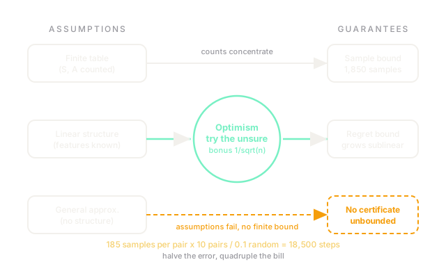
In the tabular regime, every state-action pair $(s, a)$ has its own counter and its own stored value. With $S$ states (positions the agent can be in) and $A$ actions (moves it can make), there are $S \times A$ pairs to learn, and the bounds scale with that product: more pairs, more samples, linearly. Counting visits works because each pair is visited again and again, so averages concentrate around true values by standard statistics (Hoeffding-style bounds, which you will compute below).

In the function-approximation regime, states are too many to count (pixels, sensor streams), so the agent generalizes with a model such as a linear predictor or a neural network. Generalization breaks the counting argument: visiting one state tells you something about others, but only if the function class is structured the right way. Positive results here always carry a structural assumption (linear dynamics, bounded Bellman rank, bounded eluder dimension), and the bound scales with the structure's complexity instead of $S \times A$. With no structural assumption, there is no finite guarantee at all: that is a theorem too, not a gap in the literature.

What is optimism, and why does it keep working?

Most sample-efficient algorithms share one trick: optimism in the face of uncertainty. When the agent is unsure about an action's value, it acts as if the action is as good as plausibly possible, tries it, and corrects the estimate with what it observes. An action is either good (profit) or disappointing (information that shrinks the uncertainty), so the agent cannot stay wrong for long.

Concretely, algorithms add an exploration bonus to uncertain pairs, proportional to something like $1/\sqrt{n(s,a)}$ where $n(s,a)$ is the visit count: large bonus for strangers, near zero for old friends. The bonus decays exactly as fast as the statistical uncertainty does, which is why the total regret stays bounded instead of growing forever. This is the principled cousin of the trial-and-error strategies on the exploration page: same dilemma, but the bonus is sized from the math rather than tuned by hand.

Worked mini-calculation: what does epsilon-greedy really cost?

Take a tiny tabular task: $S = 5$ states, $A = 2$ actions, so $S \times A = 10$ pairs to learn. The agent runs epsilon-greedy (it takes a random action with probability $\epsilon = 0.1$ and its current best guess otherwise) and you demand each pair's value accurate within $\eta = 0.1$ with confidence $1 - \delta = 0.95$.

Step 1, samples per pair. A standard concentration bound says $n \geq \ln(2/\delta) / (2\eta^2)$ samples pin one value down to $\pm\eta$ at confidence $1 - \delta$. Plug in: $\ln(2/0.05) = \ln(40) \approx 3.6889$, and $2\eta^2 = 2 \times 0.01 = 0.02$. So $n \geq 3.6889 / 0.02 \approx 184.44$, rounded up to 185 samples per pair.

Step 2, all pairs. Uniform coverage of 10 pairs needs $185 \times 10 =$ 1,850 well-spread samples.

Step 3, the epsilon tax. Only a fraction $\epsilon = 0.1$ of steps are random, and only random steps spread evenly, so total interaction steps come to $1{,}850 / 0.1 =$ 18,500 steps.

Read the scaling off the arithmetic: cost grows linearly with the number of pairs ($S \times A$), quadratically with $1/\eta$ (halve the error tolerance, quadruple the bill), logarithmically with $1/\delta$ (confidence is cheap), and inversely with $\epsilon$ (timid exploration multiplies the total). Tighten $\eta$ from $0.1$ to $0.01$ and the per-pair count jumps from 185 to about 18,445. That single jump explains why theory papers obsess over the accuracy parameter, and the diagram below draws this exact chain.

Code

A short script that prices the worked example above, so you can reprice it for your own numbers:

1import math2
3
4def hoeffding_samples(accuracy: float, delta: float) -> int:5    """Samples to pin one action value within accuracy at confidence 1 - delta."""6    return math.ceil(math.log(2.0 / delta) / (2.0 * accuracy**2))7
8
9def total_steps(num_pairs: int, accuracy: float, delta: float, epsilon: float) -> int:10    """Total interaction steps when only an epsilon fraction of steps spread evenly."""11    per_pair = hoeffding_samples(accuracy, delta)12    return math.ceil(per_pair * num_pairs / epsilon)13
14
15if __name__ == "__main__":16    print(hoeffding_samples(0.1, 0.05))17    print(total_steps(10, 0.1, 0.05, 0.1))

1# -> expected output:2185318500

Watch Out For

The Quick Version

• Theoretical RL prices learning: sample complexity counts steps to near-optimal behavior, regret totals the reward lost along the way, and PAC-MDP wraps the count in an explicit confidence statement.
• Tabular bounds scale with the number of state-action pairs because each pair is counted separately; function-approximation bounds scale with structural complexity and vanish entirely without a structural assumption.
• Optimism in the face of uncertainty, trying uncertain actions as if they were good, is the shared trick behind most efficient algorithms, with bonuses sized from statistics rather than tuned by hand.
• Cost scaling is concrete: for 10 pairs at accuracy 0.1 and 95 percent confidence, 185 samples per pair become 1,850 spread samples and 18,500 epsilon-greedy steps, and halving the error tolerance roughly quadruples the bill.
• A guarantee covers only its assumptions: instantiate the bound with your numbers before budgeting, and never cite a tabular certificate for an approximated agent.

What to Read Next

• Markov Decision Processes
• Exploration vs. Exploitation
• Temporal Difference Learning
• Value Iteration