Transformers in RL

Why Does This Exist?

Some tasks punish forgetfulness. You pick up a key at step 10, wander corridors for two hundred steps, then face a locked door. The right action now depends on one observation from minutes ago.

Recurrent policies handle this with a single hidden vector $h_t$ updated every step as $h_t = f(h_{t-1}, s_t)$, where $h_t$ is the memory and $s_t$ is the current state. That vector has a fixed size, so it must squeeze the whole past into a few hundred numbers. Gradients also shrink as they travel back through hundreds of updates, so the key pickup stops moving the weights. In practice the agent remembers the last room and forgets the key.

Transformers replace that bottleneck with direct lookup. The policy keeps the last $K$ tokens around (past states, actions and goal signals) and attends to all of them at once. Step 210 can pull step 10 straight in with one learned weight instead of waiting for a signal to survive two hundred squashes. That is the whole idea: attention over trajectories used as episodic memory.

This page teaches that memory mechanism: how the lookup works, why it beats recurrence on long horizons, how causal masking keeps it honest, and how goal conditioning steers it. The full return-conditioned sequence model gets its own treatment in Decision Transformers and Trajectory Transformer, which is the natural sequel. For the neural policy background, see Deep Reinforcement Learning; for the bootstrapping alternative this sidesteps, see Temporal Difference Learning.

Think of It Like This

How It Actually Works

From one hidden vector to direct lookup

A recurrent policy compresses: new observation in, old memory overwritten, one vector out. The path from step $t - 200$ to step $t$ runs through two hundred applications of the same update, and each one can dilute or overwrite the trace.

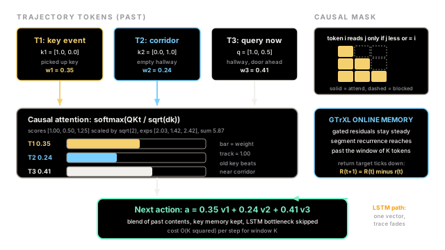
A transformer policy keeps the receipts. It stores embeddings of the last $K$ tokens and computes scaled dot-product attention at every step:

$\text{Attention}(Q, K, V) = \text{softmax}\left(\frac{QK^T}{\sqrt{d_k}}\right) V$

Here $Q$ (queries) is what the current step is looking for, $K$ (keys) is what each past token offers, $V$ (values) is the content each past token contributes, and $d_k$ is the key dimension used to keep the scores at unit scale. The output is a weighted blend of past contents, and the weights are learned. The path from any past token to the present is one direct connection, which is why a two-hundred-step dependency costs the model nothing special to reach.

The online variant you will meet by name is GTrXL. It wraps the transformer with gating on the residual connections (borrowed from recurrent gates) plus segment-level recurrence and relative positions, so the memory reaches past the current window and training stays steady where plain transformers in RL loops blew up. Think of it as the version built to survive acting and learning at the same time.

The price is compute. Attention compares every token with every other token, so a window of $K$ tokens costs $O(K^2)$ work per step. Recurrence costs $O(1)$ per step but forgets. Long memory or cheap steps: pick one.

Causal masking and goal conditioning in one sketch

Tokens are ordered in time, and the model must not peek. A causal mask $M$ is a lower-triangular matrix of ones and zeros that blanks every future position: token $i$ may read token $j$ only when $j \le i$. In code the masked scores become $-\infty$ before the softmax wherever $M_{ij} = 0$, so future tokens get exactly zero weight.

Goal conditioning steers the lookup. Instead of asking "what action is good here," the policy is handed a desired remaining return $\hat{R}_t$ (the reward still to collect this episode) alongside the state $s_t$, and predicts the action that fits both. After the environment pays reward $r_t$, the target ticks down as $\hat{R}_{t+1} = \hat{R}_t - r_t$. The full version of this trick, with trajectory token layouts and training losses, lives on the Decision Transformers and Trajectory Transformer page, so this page stops at the sketch.

Worked example: three attention weights

Say the agent stands in a hallway. Its query vector is $q = [1.0, 0.5]$. Three past tokens offer keys: $k_1 = [1.0, 0.0]$ (picked up the key two rooms back), $k_2 = [0.0, 1.0]$ (empty corridor), $k_3 = [1.0, 0.5]$ (the turn just taken). Key dimension $d_k = 2$, so the scale is $\sqrt{2} \approx 1.4142$.

Step 1, raw scores as dot products:

$s_1 = 1.0 \times 1.0 + 0.5 \times 0.0 = 1.0$ $s_2 = 1.0 \times 0.0 + 0.5 \times 1.0 = 0.5$ $s_3 = 1.0 \times 1.0 + 0.5 \times 0.5 = 1.25$

Step 2, scale by $\sqrt{d_k}$:

$[0.7071,\, 0.3536,\, 0.8839]$

Step 3, exponentiate:

$[e^{0.7071},\, e^{0.3536},\, e^{0.8839}] = [2.028,\, 1.424,\, 2.420]$

The sum is $2.028 + 1.424 + 2.420 = 5.873$. Divide through:

$w = [0.345,\, 0.243,\, 0.412]$

The policy blends past contents as $0.345\,v_1 + 0.243\,v_2 + 0.412\,v_3$, where each $v_i$ is the value content of token $i$. The recent turn gets 41 percent, the key pickup from way back still gets 35 percent, and the corridor gets 24 percent. That middle number is the point: a two-step-old event outranks a one-step-old irrelevance because the content matches, not because it is near. These are the same three weights drawn in the diagram above.

Code

The snippet below recomputes the worked example. It is the same arithmetic as the section above, so you can check the diagram against it.

1import math2from typing import List3
4
5def softmax(logits: List[float]) -> List[float]:6    """Normalizes raw scores into weights that sum to 1."""7    exps = [math.exp(s) for s in logits]8    total = sum(exps)9    return [e / total for e in exps]10
11
12def attention_weights(query: List[float], keys: List[List[float]]) -> List[float]:13    """Scaled dot-product weights of one query over past tokens."""14    dim = len(query)15    scores = [16        sum(q * k for q, k in zip(query, key)) / math.sqrt(dim) for key in keys17    ]18    return softmax(scores)19
20
21if __name__ == "__main__":22    q = [1.0, 0.5]23    keys = [[1.0, 0.0], [0.0, 1.0], [1.0, 0.5]]24    w = attention_weights(q, keys)25    print([round(v, 3) for v in w])26    assert abs(sum(w) - 1.0) < 1e-9

1# -> expected output:2[0.345, 0.243, 0.412]

Watch Out For

The Quick Version

• A transformer policy keeps its recent trajectory tokens on hand and rereads them with attention instead of squeezing the past into one recurrent vector.
• Attention output is a learned weighted blend, $\text{softmax}(QK^T / \sqrt{d_k})V$, so a step from hundreds of steps back can still win the most weight.
• A causal mask gives every token access to the past and zero access to the future, which is what keeps the policy deployable.
• Goal conditioning hands the model a remaining-return target $\hat{R}_t$ that ticks down as rewards arrive, steering which memories get used.
• GTrXL is the online-RL variant with gated residuals and segment recurrence for memory past the current window.

What to Read Next

• Decision Transformers and Trajectory Transformer
• Deep Reinforcement Learning
• Temporal Difference Learning