Decision Transformers and Trajectory Transformer
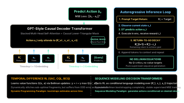
Instead of calculating values with recursive Bellman equations, Decision Transformers reframe reinforcement learning as language modeling—generating expert actions by conditioning on desired return-to-go.
Why Does This Exist?
For decades, reinforcement learning has been dominated by the dynamic programming paradigm. Algorithms like Q-learning, Actor-Critic, and policy gradients rely on temporal difference (TD) learning, updating value estimates recursively via Bellman backups:
While mathematically elegant, TD learning suffers from notorious practical instabilities in the offline (batch) setting. Bootstrapping creates a fragile feedback loop where out-of-distribution function approximation errors compound uncontrollably, causing value estimates to diverge and policies to degrade. Practitioners have had to invent complex regularization techniques—such as conservative value penalties (CQL), batch constraints (BCQ), and expectile regressions (IQL)—simply to keep temporal difference updates stable.
Meanwhile, natural language processing underwent a revolution driven by Generative Pre-trained Transformers (GPT). Large causal Transformers demonstrated that predicting the next token in a sequence using multi-head self-attention scales predictably, trains stably via standard supervised cross-entropy or mean squared error (MSE), and captures intricate long-range dependencies without any recursive value bootstrapping.
In 2021, Chen et al. introduced the Decision Transformer (DT), alongside Janner et al.'s Trajectory Transformer (TT). They proposed a radical paradigm shift: reframe reinforcement learning not as dynamic programming, but as conditional autoregressive sequence modeling. By representing an agent's experience as an interleaved sequence of return targets, states, and actions, the agent bypasses Bellman equations entirely. To act expertly, the agent simply conditions the Transformer on a high desired return-to-go and lets autoregressive self-attention generate the exact sequence of actions that yields that result.
Think of It Like This
Prompting a Mystery Novelist
Imagine you want a story where a master detective solves an impossible heist:
Traditional Reinforcement Learning (TD Learning) behaves like an accountant trying to write a novel by evaluating every sentence with a calculator. At every comma, the accountant estimates the expected book sales: "If the detective turns left, expected sales are $40,000; if they turn right, expected sales are $42,000." If the accountant's formula makes a slight overestimation error in chapter 2, that error propagates to chapter 1, corrupting the entire plot until the story falls apart.
Decision Transformer behaves like prompting an elite author (a GPT language model) with the desired ending:
"Write a thriller where the detective catches the thief, recovers the stolen diamond, and achieves a flawless 100/100 score."
The language model does not calculate expected royalty values at every word. Instead, it draws upon thousands of previously read mystery novels (the offline trajectory dataset) and generates the natural, causal sequence of actions and dialogue that logically leads to that requested 100-point climax.
Where the analogy stops: Language models predict discrete word tokens from a vocabulary. Decision Transformers handle multi-modal continuous control trajectories composed of continuous state vectors, real-valued continuous action vectors, and scalar returns-to-go, requiring separate modality projection layers and continuous regression losses.
How It Actually Works
Trajectory Representation as Token Sequences
Instead of decomposing an offline dataset into independent transition tuples , the Decision Transformer treats episodes as coherent trajectory sequences.
A trajectory of length is structured as an interleaved sequence of Return-to-Go, State, and Action tokens:
Return-to-Go ()
Rather than conditioning on the immediate reward , the model conditions on the Return-to-Go (RTG), defined as the future cumulative return remaining from timestep until the end of the episode:
Conditioning on provides a clear forward-looking objective: "What sequence of actions will accumulate reward from this state onward?"
Architecture and Causal Self-Attention
The Decision Transformer adopts a standard GPT-style causal decoder architecture:
Inputs: [ R̂₁ ] [ s₁ ] [ a₁ ] [ R̂₂ ] [ s₂ ] ──> [ â₂ ] (Predict) │ │ │ │ │Linear Proj: W_R W_s W_a W_R W_s │ │ │ │ │Pos Embed: + pos(1) + pos(1) + pos(1) + pos(2) + pos(2) ▼ ▼ ▼ ▼ ▼┌───────────────────────────────────────────────────────────────┐│ Causal Multi-Head Self-Attention ││ (Lower-Triangular Mask: Past Only) │└───────────────────────────────────────────────────────────────┘ │ ▼ Action Head W_act │ ▼ Predicted Action â₂1. Modality Embedding Projections
Because returns, states, and actions live in different vector spaces, each modality is projected into a shared embedding space of dimension :
2. Timestep Positional Embeddings
Unlike standard Transformers that use token index positions (), the Decision Transformer uses timestep embeddings based on the environment step . All three modality tokens belonging to timestep receive the same learned positional vector :
This allows the model to retain temporal alignment across the episode regardless of context truncation.
3. Causal Attention Mask
A lower-triangular causal attention mask ensures that token predictions at time only attend to historical context. Specifically, when predicting action , the model attends to:
The prediction of has access to the current state and the desired return , but never sees future states or the true action .
Training Objective and Autoregressive Rollout
Training
The model is trained entirely through supervised learning on offline trajectories sampled from dataset . For continuous action spaces, the objective is Mean Squared Error (MSE):
For discrete actions, cross-entropy loss over action logits is used. There are no critics, no target networks, and no discount factors .
Autoregressive Inference (Evaluation)
During live deployment in an environment:
- Target Specification: The user sets an initial desired target return (e.g., the maximum return in the dataset or an expert performance threshold).
- State Observation: The agent observes initial state .
- Action Generation: The prompt is passed to the Decision Transformer to predict action .
- Environment Step: The agent executes , receiving reward and transition state .
- Return-to-Go Decay: The agent decrements the return-to-go:
- Context Append: The sequence is extended with , and the process repeats autoregressively across a sliding context window of length (typically timesteps).
Contrast with Trajectory Transformer (TT)
While both models frame RL as sequence modeling, the Trajectory Transformer (Janner et al., 2021) differs fundamentally in tokenization and planning:
| Characteristic | Decision Transformer (DT) | Trajectory Transformer (TT) |
|---|---|---|
| Prediction Focus | Direct action generation conditioned on return: | Full joint distribution modeling: |
| Tokenization | Continuous linear projections per modality | Discrete tokens via uniform binning or VQ-VAE |
| Planning Mechanism | Feedforward return-conditioning at inference | Beam search planning across future predicted trajectory tokens |
| Role in RL | Policy generator (replaces actor) | Generative world model (replaces simulator and dynamics) |
Worked numerical example
Let us trace a concrete 3-step trajectory () through return-to-go calculation, context windowing, action loss computation, and inference decay.
Step 1: Compute Returns-to-Go
Suppose a demonstrated trajectory yields rewards:
The total cumulative return is .
The return-to-go for each step is computed backward:
Step 2: Context Input at Timestep
At timestep , the causal context sequence presented to the Transformer consists of 5 tokens:
The Transformer processes these 5 tokens through causal self-attention. The query vector at the final position () attends to all 5 tokens to output the predicted action vector .
Step 3: Compute Action Prediction Loss
Suppose the true 2-dimensional continuous action in the dataset is:
The Decision Transformer's linear action head outputs prediction:
The Mean Squared Error (MSE) loss is evaluated:
This supervised gradient updates and the self-attention weights via standard Adam optimizer steps.
Step 4: Inference Return-to-Go Decay
During real-time evaluation:
- The user specifies target return .
- The agent executes predicted action in the environment.
- The environment emits reward .
- The agent updates its prompt return-to-go for step :
The agent's internal goal is dynamically updated: it now knows that to satisfy the requested 10.0 overall performance, it must collect exactly 8.0 remaining points over the remainder of the episode.
Code
Below is a self-contained, type-hinted Python implementation of the core Decision Transformer trajectory evaluation engine, including return-to-go computation, causal attention masking, continuous action MSE loss, and autoregressive return decay:
from dataclasses import dataclassimport mathfrom typing import List, Tuple
@dataclassclass TrajectoryToken: """Represents an individual token in the interleaved trajectory sequence."""
modality: str # 'RTG', 'STATE', or 'ACTION' timestep: int value: float
class DecisionTransformerTrajectoryEvaluator: """Evaluates trajectory tokenization, causal masking, return-to-go decay, and action prediction loss."""
def __init__(self, embedding_dim: int = 16) -> None: self.embedding_dim = embedding_dim
def compute_returns_to_go(self, rewards: List[float]) -> List[float]: """Computes Return-to-go R_hat_t = sum_{t'=t}^T r_{t'} for each timestep.""" t_len = len(rewards) rtg = [0.0] * t_len running_sum = 0.0 for i in reversed(range(t_len)): running_sum += rewards[i] rtg[i] = running_sum return rtg
def construct_token_sequence( self, returns_to_go: List[float], states: List[List[float]], actions: List[List[float]], ) -> List[TrajectoryToken]: """Constructs interleaved token sequence: (R_hat_1, s_1, a_1, R_hat_2, s_2, a_2, ...).""" tokens: List[TrajectoryToken] = [] for t in range(len(returns_to_go)): step_idx = t + 1 tokens.append(TrajectoryToken("RTG", step_idx, returns_to_go[t])) tokens.append(TrajectoryToken("STATE", step_idx, states[t][0])) tokens.append(TrajectoryToken("ACTION", step_idx, actions[t][0])) return tokens
def build_causal_mask(self, num_tokens: int) -> List[List[int]]: """Builds lower-triangular causal attention mask (1 = attend, 0 = mask).""" mask = [ [1 if j <= i else 0 for j in range(num_tokens)] for i in range(num_tokens) ] return mask
def compute_action_loss_mse( self, pred_action: List[float], target_action: List[float] ) -> float: """Computes Mean Squared Error loss between predicted and ground-truth action vectors.""" assert len(pred_action) == len(target_action) dim = len(pred_action) sq_diff_sum = sum( (p - t) ** 2 for p, t in zip(pred_action, target_action) ) return sq_diff_sum / dim
def step_inference_rtg( self, current_rtg: float, received_reward: float ) -> float: """Updates return-to-go for the next timestep: R_hat_{t+1} = R_hat_t - r_t.""" return current_rtg - received_reward
if __name__ == "__main__": evaluator = DecisionTransformerTrajectoryEvaluator()
# 1. Worked Numerical Example: T=3 trajectory rewards = [2.0, 3.0, 5.0] rtg = evaluator.compute_returns_to_go(rewards)
print("=== Returns-to-Go Calculation ===") print(f"Step Rewards: {rewards}") print(f"Returns-to-Go: {rtg}") assert rtg == [10.0, 8.0, 5.0]
# 2. Context at t=2: Action Loss Evaluation pred_a2 = [0.45, 0.85] gt_a2 = [0.50, 0.80] mse_loss = evaluator.compute_action_loss_mse(pred_a2, gt_a2)
print("\n=== Action Prediction Loss (MSE) ===") print(f"Predicted Action a_hat_2: {pred_a2}") print(f"Ground Truth Action a_2: {gt_a2}") print(f"MSE Loss: {mse_loss:.6f}") assert math.isclose(mse_loss, 0.0025)
# 3. Inference RTG Decay # Starting at R_hat_1 = 10.0, agent executes a_1 and receives r_1 = 2.0 rtg_t2 = evaluator.step_inference_rtg( current_rtg=rtg[0], received_reward=rewards[0] ) print("\n=== Inference Return-to-Go Decay ===") print( f"Prompt RTG at t=2: R_hat_2 = R_hat_1 - r_1 = {rtg[0]} - {rewards[0]} = {rtg_t2:.1f}" ) assert math.isclose(rtg_t2, 8.0)
# 4. Token Sequence and Causal Mask Verification mock_states = [[1.0], [1.2], [1.5]] mock_actions = [[0.5], [0.8], [0.9]] tokens = evaluator.construct_token_sequence(rtg, mock_states, mock_actions) causal_mask = evaluator.build_causal_mask(len(tokens))
print("\n=== Causal Mask Verification ===") print(f"Total Trajectory Tokens (3 steps x 3 modalities): {len(tokens)}") print(f"Token 0 ({tokens[0].modality}_1) attend vector: {causal_mask[0]}") print(f"Token 4 ({tokens[4].modality}_2) attend vector: {causal_mask[4]}")
assert len(tokens) == 9 assert causal_mask[0] == [1, 0, 0, 0, 0, 0, 0, 0, 0] assert causal_mask[4] == [1, 1, 1, 1, 1, 0, 0, 0, 0] print("\nAll Decision Transformer assertions passed successfully!")Expected output:
=== Returns-to-Go Calculation ===Step Rewards: [2.0, 3.0, 5.0]Returns-to-Go: [10.0, 8.0, 5.0]
=== Action Prediction Loss (MSE) ===Predicted Action a_hat_2: [0.45, 0.85]Ground Truth Action a_2: [0.5, 0.8]MSE Loss: 0.002500
=== Inference Return-to-Go Decay ===Prompt RTG at t=2: R_hat_2 = R_hat_1 - r_1 = 10.0 - 2.0 = 8.0
=== Causal Mask Verification ===Total Trajectory Tokens (3 steps x 3 modalities): 9Token 0 (RTG_1) attend vector: [1, 0, 0, 0, 0, 0, 0, 0, 0]Token 4 (STATE_2) attend vector: [1, 1, 1, 1, 1, 0, 0, 0, 0]
All Decision Transformer assertions passed successfully!Watch Out For
The Trajectory Stitching Failure Mode
The Trap: In offline RL benchmarks (such as D4RL AntMaze), an agent often needs to "stitch" parts of multiple suboptimal trajectories. For example, trajectory 1 demonstrates navigating from start to checkpoint , while trajectory 2 demonstrates navigating from to goal . Temporal difference algorithms (like CQL or IQL) excel at this: Bellman updates propagate value backwards across states, stitching and together into an optimal policy.
Because the vanilla Decision Transformer performs conditional sequence matching rather than dynamic programming, it cannot stitch fragments without having observed complete trajectories. If the dataset only contains separate, mediocre trajectories with low returns, prompting the model with an expert return forces the Transformer out-of-distribution. Instead of discovering an optimal path, the model outputs erratic, uncoordinated actions.
The Symptom: Decision Transformer achieves state-of-the-art performance on continuous locomotion tasks (Gym MuJoCo Hopper/HalfCheetah) where datasets contain smooth, near-expert trajectories, but scores near zero on sparse-reward navigation tasks (AntMaze) that strictly require trajectory stitching.
The Fix:
- Hybridize with Value Learning: Use Q-guided Decision Transformers (Q-DT) or Dual-Value Transformers where token sampling is guided by learned temporal-difference critic evaluations.
- Data Augmentation: Augment the offline dataset using conservative model rollouts or sub-trajectory recombination before training.
- Trajectory Transformer with Beam Search: Use the Trajectory Transformer (TT) instead of DT; because TT explicitly models transition dynamics , beam search planning can stitch disjoint paths during inference.
The Quick Version
- RL as Sequence Modeling: Decision Transformer replaces recursive Bellman backups with conditional autoregressive sequence modeling, using a GPT-style causal decoder to predict actions from historical context.
- Interleaved Trajectory Tokens: Episodes are structured as token triplets paired with timestep embeddings, where Return-to-Go provides the forward conditioning target.
- Pure Supervised Training: The model is trained using standard mean squared error (continuous actions) or cross-entropy (discrete actions), eliminating target networks, value critics, and offline Bellman instability.
- Inference via Return Decay: The agent is prompted with a desired high return and decrements the target dynamically after each environment reward (), guiding the Transformer to fulfill the overall episode objective.