Transition Dynamics
Transition dynamics define the probability distribution over where an agent will end up next after taking an action in a given state, modeling the uncertain physics of the environment.
Why Does This Exist?
In idealized computing environments, taking an action produces a deterministic outcome: if you write a byte to memory, it lands in that memory address with certainty. Real physical systems and competitive environments rarely behave this predictably. A robot issuing a drive command may hit slippery ice, an autonomous car steering right can encounter sudden wind gusts or traction loss, a network router forwarding a packet may suffer buffer drops, and a trading algorithm submitting a market order faces slippage and stochastic order fills.
Without a formal mechanism for transition dynamics, decision algorithms assume deterministic transitions—that taking action in state always leads to a single known next state . Under this naive assumption, an agent designs brittle plans that catastrophic noise dismantles within milliseconds. Furthermore, foundational reinforcement learning frameworks—such as Markov Decision Processes, Bellman Equations, and Value Functions—cannot formulate expected returns without knowing how likely each outcome is.
Transition dynamics provide the exact mathematical engine that models environmental physics. By mapping each state-action pair to a rigorous probability distribution over all possible successor states , the dynamics function lets an agent compute expected returns, hedge against downside risks, and plan optimal behaviors in uncertain worlds.
Think of It Like This
Driving on an icy road
Imagine driving down a winter highway approaching an intersection. You turn your steering wheel 30 degrees to the right: that physical command is your action , and your current vehicle position and velocity make up your state .
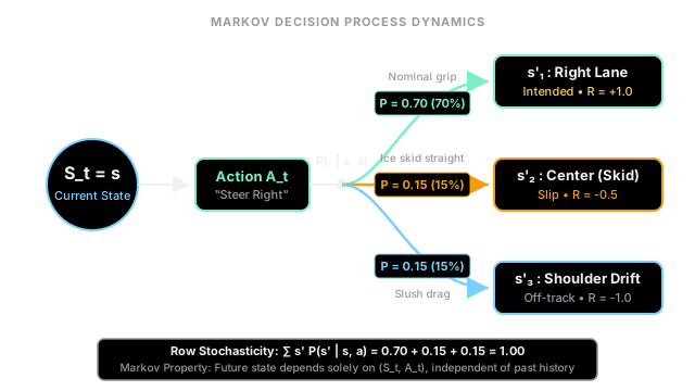
On dry, clean asphalt, your steering input determines your next state with near 100% certainty: you cleanly enter the right lane. But on an icy road, traction physics decouples your intention from the physical outcome. Turning the wheel right produces a probability distribution:
- 70% probability: The front tires bite through the frost and track into the right lane ().
- 15% probability: The front wheels lose grip entirely, and momentum skids the vehicle straight forward into the center of the intersection ().
- 15% probability: Road slush catches the left tires, pulling the car onto the shoulder ().
You do not control which of these three outcomes occurs on any single attempt. The icy road, the tire rubber, and the laws of friction—the environment dynamics—decide the actual successor state. Your only lever of control is choosing which action distribution to gamble on.
Where the analogy stops: A human driver continuously corrects their steering in real time using high-frequency sensory feedback. In a discrete-time Markov process, the agent must commit to a single discrete action for the duration of the time step, and the transition kernel samples the successor state in one atomic transition before the agent receives its next observation.
How It Actually Works
The Conditional Dynamics Kernel and Joint Dynamics Function
In a Markov Decision Process, the environment's physics are formalized through conditional probability distributions. Let denote the set of all valid states, denote the set of all actions, and denote the set of possible rewards.
1. State Transition Probability Function
The standard state transition probability (often written as or ) defines the conditional probability that the environment transitions to state at time , given that the agent observed state and selected action at time :
This formulation relies on the Markov Property: the transition distribution depends exclusively on the current state and immediate action , making the full historical sequence of prior states and actions conditionally independent:
2. The Four-Argument Joint Dynamics Function
In modern literature (notably Sutton & Barto), the environment is completely characterized by a four-argument joint dynamics function :
The state transition probability is recovered by marginalizing out the reward:
Similarly, the expected immediate reward received from taking action in state is the expectation across all possible rewards and successor states:
3. Row Stochasticity and Transition Matrices
Because represents a valid probability distribution over mutual events, it must satisfy the axioms of probability:
For a finite state space with , each action defines an transition probability matrix :
Every row of sums to exactly 1, making a right-stochastic matrix. If the agent follows a fixed policy , the induced transition matrix is:
Given an initial state probability distribution vector , the state distribution at step evolves through vector-matrix multiplication:
Worked numerical example
Consider a 3-state stochastic corridor environment:
- : Safe Road
- : Icy Patch
- : Goal Destination (absorbing terminal state)
The agent chooses action . The transition dynamics matrix is:
Row checks confirm row-stochasticity:
- Row 1:
- Row 2:
- Row 3:
Step 1: Forward distribution propagation over time
Assume the agent starts with absolute certainty in , giving initial state vector:
After 1 step, the state distribution is:
After 2 steps, the distribution becomes:
Notice that the sum , preserving the total probability mass, with a 57% chance of already having reached the Goal.
Step 2: Weighting Bellman value expectations
Now let current state values be estimated as:
Taking action from yields an immediate step reward , with discount factor . The expected successor state value is computed by weighting each possible future state by its transition probability:
The Bellman action-value is therefore:
Without the transition probabilities , computing this expectation would be impossible.
Code
import randomfrom typing import Dict, List, Tuple
class TransitionModel: """Represents an MDP transition dynamics kernel P(s' | s, a) with invariant verification."""
def __init__( self, states: List[str], actions: List[str], transitions: Dict[Tuple[str, str], Dict[str, float]], ) -> None: self.states = states self.actions = actions self.transitions = transitions self._validate_stochasticity()
def _validate_stochasticity(self, tolerance: float = 1e-6) -> None: """Verifies row-stochasticity: for every (s, a), sum_s' P(s'|s,a) == 1.0.""" for s in self.states: for a in self.actions: dist = self.transitions.get((s, a), {}) total_prob = sum(dist.values()) if abs(total_prob - 1.0) > tolerance: raise ValueError( f"Row-stochasticity violated for ({s}, {a}): sum = {total_prob:.6f}" ) for s_prime, prob in dist.items(): if prob < 0.0 or prob > 1.0: raise ValueError( f"Invalid probability {prob} for transition ({s}, {a}) -> {s_prime}" )
def transition_matrix(self, action: str) -> List[List[float]]: """Constructs the square transition matrix P^a where entry (i, j) is P(s_j | s_i, a).""" return [ [self.transitions[(s, action)].get(s_next, 0.0) for s_next in self.states] for s in self.states ]
def sample_next_state(self, state: str, action: str, rng: random.Random) -> str: """Simulates environment physics by sampling s' ~ P(. | s, a).""" dist = self.transitions[(state, action)] candidates = list(dist.keys()) weights = list(dist.values()) return rng.choices(candidates, weights=weights, k=1)[0]
def propagate_distribution( distribution: List[float], transition_matrix: List[List[float]]) -> List[float]: """Computes mu_{t+1} = mu_t @ P for a state distribution vector mu.""" n_states = len(transition_matrix) return [ sum(distribution[i] * transition_matrix[i][j] for i in range(n_states)) for j in range(n_states) ]
if __name__ == "__main__": # Define states and actions for a 3-state icy corridor states = ["SafeRoad", "IcyPatch", "Goal"] actions = ["Forward"]
# Dynamics mapping: (state, action) -> {next_state: probability} transitions = { ("SafeRoad", "Forward"): {"SafeRoad": 0.10, "IcyPatch": 0.70, "Goal": 0.20}, ("IcyPatch", "Forward"): {"SafeRoad": 0.20, "IcyPatch": 0.30, "Goal": 0.50}, ("Goal", "Forward"): {"SafeRoad": 0.00, "IcyPatch": 0.00, "Goal": 1.00}, }
env = TransitionModel(states, actions, transitions) p_mat = env.transition_matrix("Forward")
# 1. Exact theoretical distribution evolution: mu_{t+1} = mu_t @ P mu_0 = [1.0, 0.0, 0.0] # Agent begins in SafeRoad with certainty print("Initial distribution (t=0):", [round(p, 4) for p in mu_0])
mu_1 = propagate_distribution(mu_0, p_mat) print("Step 1 distribution (t=1):", [round(p, 4) for p in mu_1])
mu_2 = propagate_distribution(mu_1, p_mat) print("Step 2 distribution (t=2):", [round(p, 4) for p in mu_2])
# 2. Monte Carlo environment sampling: draw 10,000 transitions from SafeRoad rng = random.Random(42) sample_counts = {s: 0 for s in states} trials = 10000
for _ in range(trials): s_prime = env.sample_next_state("SafeRoad", "Forward", rng) sample_counts[s_prime] += 1
empirical_dist = {s: round(count / trials, 4) for s, count in sample_counts.items()} print("\nEmpirical frequencies after 10,000 trials from SafeRoad:") print(empirical_dist)
# 3. Bellman expectation evaluation: E[V(S_{t+1}) | S_t = SafeRoad, A_t = Forward] state_values = {"SafeRoad": 2.0, "IcyPatch": 5.0, "Goal": 10.0} reward = -1.0 gamma = 0.90
expected_next_v = sum( prob * state_values[s_next] for s_next, prob in transitions[("SafeRoad", "Forward")].items() ) q_value = reward + gamma * expected_next_v
print(f"\nExpected successor value E[V(S')]: {expected_next_v:.2f}") print(f"Action value Q(SafeRoad, Forward): {q_value:.2f}")
# Explicit test assertions assert round(mu_1[1], 2) == 0.70, "Step 1 IcyPatch probability must equal 0.70" assert round(mu_2[2], 2) == 0.57, "Step 2 Goal probability must equal 0.57" assert round(q_value, 2) == 4.13, "Q-value must equal 4.13"Initial distribution (t=0): [1.0, 0.0, 0.0]Step 1 distribution (t=1): [0.1, 0.7, 0.2]Step 2 distribution (t=2): [0.15, 0.28, 0.57]
Empirical frequencies after 10,000 trials from SafeRoad:{'SafeRoad': 0.0986, 'IcyPatch': 0.7045, 'Goal': 0.1969}
Expected successor value E[V(S')]: 5.70Action value Q(SafeRoad, Forward): 4.13Watch Out For
Assuming deterministic transitions in real-world systems
A common pitfall is constructing simulators or planning models that treat physics as deterministic ( for a single successor state). When algorithms like Monte Carlo Tree Search (MCTS) or Value Iteration plan under deterministic dynamics, they find fragile policies that cut hair-thin margins next to hazards (e.g. driving right along a cliff edge because the planned path technically never touches it).
When transferred to physical hardware, micro-disturbances, motor friction variances, wind resistance, and sensor latency disrupt the intended trajectory, causing catastrophic failure. To prevent this sim-to-real gap, practitioners must explicitly incorporate transition stochasticity through domain randomization (randomly jittering friction, mass, and delay parameters during rollout generation), using robust MDP formulations, or enforcing entropy-regularized exploration.
Violating the row-stochasticity constraint
When building custom simulators, learning environment dynamics with neural networks, or manually designing transition probability tables, practitioners frequently introduce subtle normalization errors where rows do not sum to unity () or produce negative probability mass.
If row sums exceed 1.0, Bellman updates artificially inflate future value estimates, causing value functions to diverge to positive infinity. Conversely, if row sums fall below 1.0, probability mass leaks on every iteration, shrinking value estimates as if an artificial discount were applied. For learned dynamics models, always apply a strictly normalized softmax projection over successor state logits:
In tabular environments, add assertion checks confirming that every row sums to and contains zero negative elements.
The Quick Version
- Transition dynamics govern the environment's physics by assigning a probability distribution over all possible next states given the current state and chosen action.
- The Markov property guarantees that future transitions depend solely on the current state-action pair , making the preceding trajectory history conditionally independent.
- Every valid transition matrix must be row-stochastic: all probabilities must be non-negative and every row must sum to exactly ().
- Transition dynamics weight future value estimates during Bellman updates; model-based RL plans directly with , while model-free methods sample from it via experience.