Trust Region and Proximal Methods

Trust region and proximal methods constrain policy updates within a mathematically bounded statistical distance, preventing catastrophic policy collapse while guaranteeing monotonic performance improvements.

Trust region methods constrain policy updates within a statistical KL divergence sphere to prevent policy collapse and guarantee monotonic improvement.

Why Does This Exist?

In supervised learning, an aggressive gradient update that overshoots slightly increases the loss for a single training batch. Crucially, the underlying dataset remains fixed and stationary; subsequent mini-batches simply correct the error.

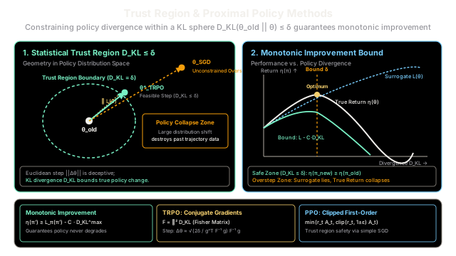
In reinforcement learning, the situation is precarious because the policy generates its own training data. If a gradient step changes the parameter vector $\boldsymbol{\theta}$ too drastically, the resulting policy $\pi_{\boldsymbol{\theta}}$ shifts unpredictably in output action distribution space:

The Catastrophic Step Problem: A bad gradient step causes the policy to begin selecting destructive actions. The agent immediately falls into low-reward, unrecoverable regions of the state space. Because the agent can now only collect trajectories from this degraded policy, the new training data contains exclusively poor outcomes, causing permanent and irreversible policy collapse.
The Deception of Euclidean Parameter Space: In deep neural networks, Euclidean distance between weight vectors $\|\boldsymbol{\theta}_{\text{new}} - \boldsymbol{\theta}_{\text{old}}\|_2$ is completely disconnected from the actual change in the policy distribution. In a sensitive hidden layer with saturated activations, a microscopic parameter change $\Delta \boldsymbol{\theta} = 0.001$ can flip the output policy from choosing Action A with $99\%$ probability to choosing Action B with $99\%$ probability. Conversely, in a wide layer with dead neurons, a large shift $\Delta \boldsymbol{\theta} = 1.0$ might cause zero noticeable change.

Standard policy gradient algorithms (such as REINFORCE or Vanilla Actor-Critic) optimize in Euclidean parameter space without accounting for this geometry. Trust region and proximal methods solve this by enforcing optimization constraints directly in probability distribution space using Kullback-Leibler (KL) divergence. By bounding how much the output action distribution is permitted to deviate, these methods provide a mathematical guarantee of monotonic policy improvement.

Think of It Like This

Navigating a Foggy Mountain Ridge: The Safety Tether

Imagine hiking along a knife-edge mountain ridge completely enveloped in dense fog:

Standard Policy Gradient (Unconstrained Leap): You feel the terrain sloping upward directly under your boots (the local policy gradient $\nabla_{\boldsymbol{\theta}} J$ ). Confident in this local slope, you take a bold, running leap forward. But five meters ahead, the ridge ends in a sheer, vertical precipice hidden by the fog. You plunge into the canyon. In reinforcement learning, that precipice is catastrophic policy collapse: your weights changed so much that your agent lost the ability to balance, and because it cannot balance, it can never collect the data required to learn how to balance again.
Trust Region Policy Optimization (The Steel Safety Tether): Before taking any step, you secure a high-tensile steel safety tether anchored to your last confirmed safe footing ( $\boldsymbol{\theta}_{\text{old}}$ ) with an exact maximum radius of $\delta$ (the KL divergence constraint $\bar{D}_{\text{KL}} \le \delta$ ). You are strictly forbidden from stepping outside that sphere. Because your local terrain map is mathematically guaranteed to be accurate within that radius, you can maximize your elevation gain safely without ever risking a fatal fall.
Proximal Policy Optimization (The Elastic Harness): Rather than solving an expensive quadratic constraint equation to build a rigid steel tether, PPO equips you with an elastic harness that gently clips your stride. If you attempt to step outside the safe $[1 - \epsilon, 1 + \epsilon]$ window, the harness removes any incentive to step further, achieving trust-region safety with standard walking mechanics.

Where the analogy stops: A mountain tether measures physical distance in meters. A trust region in RL measures statistical divergence (relative entropy) across policy action probability distributions averaged over the entire state space of the Markov Decision Process.

How It Actually Works

The Monotonic Improvement Theory and Trust Region Formulation

The theoretical foundation of modern trust region policy search was established by Kakade and Langford (2002) and operationalized for deep neural networks by Schulman et al. in Trust Region Policy Optimization (TRPO, 2015).

1+-----------------------------------------------------------------------------------------+2|                         TRUST REGION & PROXIMAL OPTIMIZATION PARADIGM                   |3+-----------------------------------------------------------------------------------------+4| Performance Identity  | η(π_new) = η(π_old) + E_{s~ρ, a~π_new} [ A^{π_old}(s, a) ]       |5| Surrogate Objective   | L(θ) = E_{s~ρ_old, a~π_old} [ (π_θ(a|s) / π_old(a|s)) · A(s, a) ]|6| Monotonic Bound       | η(π_new) ≥ L(π_new) - C · D_KL^max(π_old, π_new)                |7| TRPO Formulation      | max_θ L(θ)   subject to   E_s [ D_KL(π_old || π_θ) ] ≤ δ        |8| PPO-Clip Formulation  | max_θ E_t [ min( r_t(θ) A_t,  clip(r_t(θ), 1±ε) A_t ) ]          |9+-----------------------------------------------------------------------------------------+

1. The Relative Performance Identity

Let $\eta(\pi) = \mathbb{E}_{\tau \sim \pi} \left[ \sum_{t=0}^{\infty} \gamma^t r_t \right]$ denote the expected discounted return of policy $\pi$ . Kakade and Langford proved that the performance of a new policy $\pi_{\text{new}}$ can be related exactly to an old policy $\pi_{\text{old}}$ via:

\eta(\pi_{\text{new}}) = \eta(\pi_{\text{old}}) + \mathbb{E}_{s \sim \rho_{\pi_{\text{new}}}, \, a \sim \pi_{\text{new}}} \left[ A^{\pi_{\text{old}}}(s, a) \right]

where $\rho_\pi(s) = \sum_{t=0}^{\infty} \gamma^t P(S_t = s \mid \pi)$ is the discounted state visitation distribution under $\pi$ , and $A^{\pi_{\text{old}}}(s, a)$ is the advantage function.

2. The Local Surrogate Objective

Evaluating the exact expectation in the performance identity requires sampling states from $\rho_{\pi_{\text{new}}}$ , which is impossible before the new policy is chosen. TRPO replaces $\rho_{\pi_{\text{new}}}$ with the known, sampled state distribution $\rho_{\pi_{\text{old}}}$ , yielding the surrogate objective $L_{\pi_{\text{old}}}(\pi_{\text{new}})$ :

L_{\pi_{\text{old}}}(\pi_{\text{new}}) = \eta(\pi_{\text{old}}) + \sum_{s} \rho_{\pi_{\text{old}}}(s) \sum_{a} \pi_{\text{new}}(a \mid s) A^{\pi_{\text{old}}}(s, a)

Using importance sampling, this can be written as an empirical expectation over trajectories collected under $\pi_{\text{old}}$ :

L_{\boldsymbol{\theta}_{\text{old}}}(\boldsymbol{\theta}) = \mathbb{E}_{s \sim \rho_{\boldsymbol{\theta}_{\text{old}}}, \, a \sim \pi_{\boldsymbol{\theta}_{\text{old}}}} \left[ \frac{\pi_{\boldsymbol{\theta}}(a \mid s)}{\pi_{\boldsymbol{\theta}_{\text{old}}}(a \mid s)} A^{\pi_{\boldsymbol{\theta}_{\text{old}}}}(s, a) \right]

Notice that at $\boldsymbol{\theta} = \boldsymbol{\theta}_{\text{old}}$ , the surrogate objective matches the true performance: $L_{\boldsymbol{\theta}_{\text{old}}}(\boldsymbol{\theta}_{\text{old}}) = \eta(\boldsymbol{\theta}_{\text{old}})$ , and their first derivatives are identical: $\nabla_{\boldsymbol{\theta}} L(\boldsymbol{\theta})\big|_{\boldsymbol{\theta}_{\text{old}}} = \nabla_{\boldsymbol{\theta}} \eta(\boldsymbol{\theta})\big|_{\boldsymbol{\theta}_{\text{old}}}$ .

3. The Monotonic Improvement Theorem

Schulman et al. proved that true return is lower-bounded by the surrogate objective minus a penalty proportional to the maximum KL divergence:

\eta(\pi_{\text{new}}) \ge L_{\pi_{\text{old}}}(\pi_{\text{new}}) - C \cdot D_{\text{KL}}^{\max}(\pi_{\text{old}}, \pi_{\text{new}})

where the constant $C$ is defined by:

C = \frac{4 \epsilon \gamma}{(1 - \gamma)^2}, \quad \text{with } \epsilon = \max_{s, a} \left| A^{\pi_{\text{old}}}(s, a) \right|

This bound guarantees that any policy update $\pi_{\text{new}}$ that increases the right-hand side is guaranteed to monotonically improve true performance: $\eta(\pi_{\text{new}}) \ge \eta(\pi_{\text{old}})$ .

4. The TRPO Constrained Optimization Problem

Because the theoretical constant $C$ is extremely large (demanding impractically small step sizes), TRPO replaces the penalty with a strict trust region constraint:

\max_{\boldsymbol{\theta}} \; L_{\boldsymbol{\theta}_{\text{old}}}(\boldsymbol{\theta}) \quad \text{subject to} \quad \bar{D}_{\text{KL}}(\boldsymbol{\theta}_{\text{old}}, \boldsymbol{\theta}) \le \delta

where $\bar{D}_{\text{KL}}(\boldsymbol{\theta}_{\text{old}}, \boldsymbol{\theta}) = \mathbb{E}_{s \sim \rho_{\boldsymbol{\theta}_{\text{old}}}} \left[ D_{\text{KL}}(\pi_{\boldsymbol{\theta}_{\text{old}}}(\cdot \mid s) \parallel \pi_{\boldsymbol{\theta}}(\cdot \mid s)) \right]$ .

To solve this constrained problem with deep neural networks:

Linearize the objective: $L(\boldsymbol{\theta}) \approx L(\boldsymbol{\theta}_{\text{old}}) + \mathbf{g}^\top (\boldsymbol{\theta} - \boldsymbol{\theta}_{\text{old}})$ , where $\mathbf{g} = \nabla_{\boldsymbol{\theta}} L$ .
Quadratic approximation of the constraint: $\bar{D}_{\text{KL}}(\boldsymbol{\theta}_{\text{old}}, \boldsymbol{\theta}) \approx \frac{1}{2} (\boldsymbol{\theta} - \boldsymbol{\theta}_{\text{old}})^\top \mathbf{F} (\boldsymbol{\theta} - \boldsymbol{\theta}_{\text{old}})$ , where $\mathbf{F}$ is the Fisher Information Matrix $\mathbf{F} = \nabla_{\boldsymbol{\theta}}^2 \bar{D}_{\text{KL}}$ .
The optimal analytical update direction is the Natural Policy Gradient: $\boldsymbol{\theta} - \boldsymbol{\theta}_{\text{old}} = \sqrt{\frac{2 \delta}{\mathbf{g}^\top \mathbf{F}^{-1} \mathbf{g}}} \mathbf{F}^{-1} \mathbf{g}$
Because inverting $\mathbf{F} \in \mathbb{R}^{d \times d}$ is impossible for millions of parameters, TRPO uses the Conjugate Gradient algorithm to compute $\mathbf{x} \approx \mathbf{F}^{-1} \mathbf{g}$ via Hessian-vector products without ever storing $\mathbf{F}$ , followed by a backtracking line search.

5. Proximal Policy Optimization (PPO)

While TRPO guarantees stability, its second-order Conjugate Gradient machinery is computationally expensive. Proximal Policy Optimization (PPO) approximates the trust region using a purely first-order clipped objective:

L^{\text{CLIP}}(\boldsymbol{\theta}) = \hat{\mathbb{E}}_t \left[ \min\left( r_t(\boldsymbol{\theta}) \hat{A}_t, \; \text{clip}(r_t(\boldsymbol{\theta}), 1 - \epsilon, 1 + \epsilon) \hat{A}_t \right) \right]

where probability ratio $r_t(\boldsymbol{\theta}) = \frac{\pi_{\boldsymbol{\theta}}(a_t \mid s_t)}{\pi_{\boldsymbol{\theta}_{\text{old}}}(a_t \mid s_t)}$ . If the policy changes so much that $r_t(\boldsymbol{\theta})$ strays outside $[1 - \epsilon, 1 + \epsilon]$ , the clipping term removes the gradient incentive, providing trust region stability via standard stochastic gradient descent.

Worked numerical example

Let us trace how trust region constraints evaluate and filter policy updates on a single state $s$ with two actions $\mathcal{A} = \{a_1, a_2\}$ .

1. Setup Parameters

Old Policy: $\boldsymbol{\pi}_{\text{old}} = [0.80, 0.20]^\top$ .
Advantage Values: $A(s, a_1) = +0.50$ , $A(s, a_2) = -2.00$ .
Verify that the old policy has zero expected advantage: $\sum_{a} \pi_{\text{old}}(a) A(s, a) = (0.80)(+0.50) + (0.20)(-2.00) = +0.40 - 0.40 = 0.00$
Trust Region Bound: $\delta = 0.010$ .

2. Evaluating Candidate Policy 1 (Safe Trust Region Step)

Consider a conservative candidate policy: $\boldsymbol{\pi}_1 = [0.85, 0.15]^\top$ .

Surrogate Improvement: $\Delta L_1 = \sum_{a} \pi_1(a) A(s, a) = (0.85)(+0.50) + (0.15)(-2.00) = 0.425 - 0.300 = +0.125$
Kullback-Leibler Divergence: $D_{\text{KL}}(\boldsymbol{\pi}_{\text{old}} \parallel \boldsymbol{\pi}_1) = 0.80 \ln\left(\frac{0.80}{0.85}\right) + 0.20 \ln\left(\frac{0.20}{0.15}\right)$ $\ln\left(\frac{0.80}{0.85}\right) = \ln(0.941176) \approx -0.060625 \implies 0.80 \times (-0.060625) \approx -0.048500$ $\ln\left(\frac{0.20}{0.15}\right) = \ln(1.333333) \approx +0.287682 \implies 0.20 \times (+0.287682) \approx +0.057536$ $D_{\text{KL}}(\boldsymbol{\pi}_{\text{old}} \parallel \boldsymbol{\pi}_1) = -0.048500 + 0.057536 = 0.009036$
Trust Region Feasibility Check: $0.009036 \le 0.010 \quad \implies \quad \textbf{FEASIBLE (ACCEPTED)}$ Candidate 1 provides a safe, verified performance improvement of $+0.1250$ while strictly respecting the trust region boundary.

3. Evaluating Candidate Policy 2 (Destructive Overstep)

Consider an aggressive, unconstrained policy that pushes action $a_1$ to near certainty: $\boldsymbol{\pi}_2 = [0.98, 0.02]^\top$ .

Surrogate Improvement: $\Delta L_2 = (0.98)(+0.50) + (0.02)(-2.00) = 0.490 - 0.040 = +0.450$ The local surrogate objective predicts an apparent major improvement of $+0.4500$ .
Kullback-Leibler Divergence: $D_{\text{KL}}(\boldsymbol{\pi}_{\text{old}} \parallel \boldsymbol{\pi}_2) = 0.80 \ln\left(\frac{0.80}{0.98}\right) + 0.20 \ln\left(\frac{0.20}{0.02}\right)$ $\ln\left(\frac{0.80}{0.98}\right) = \ln(0.816327) \approx -0.202941 \implies 0.80 \times (-0.202941) \approx -0.162353$ $\ln\left(\frac{0.20}{0.02}\right) = \ln(10.000) \approx +2.302585 \implies 0.20 \times (+2.302585) \approx +0.460517$ $D_{\text{KL}}(\boldsymbol{\pi}_{\text{old}} \parallel \boldsymbol{\pi}_2) = -0.162353 + 0.460517 = 0.298164$
Trust Region Feasibility Check: $0.298164 \gg 0.010 \quad \implies \quad \textbf{INFEASIBLE (REJECTED)}$ Candidate 2 violates the trust region by nearly 30x. While the local surrogate predicted an apparent $+0.450$ gain, in reality the state distribution $\rho_\pi(s)$ across the MDP collapses, resulting in catastrophic failure. The trust region constraint rejects Candidate 2.

Code

The following self-contained Python script implements a TrustRegionOptimizer that computes surrogate objective gains, exact KL divergences, evaluates candidate policy proposals against the trust region bound $\delta$ , and selects the optimal verified step with automated assertions.

1from typing import List, Tuple2import numpy as np3
4
5class TrustRegionOptimizer:6    """Evaluates policy candidates under surrogate objectives and KL trust region constraints."""7
8    def __init__(9        self,10        pi_old: np.ndarray,11        advantages: np.ndarray,12        delta_kl: float = 0.01,13        gamma: float = 0.99,14    ) -> None:15        self.pi_old = np.asarray(pi_old, dtype=np.float64)16        self.advantages = np.asarray(advantages, dtype=np.float64)17        self.delta_kl = delta_kl18        self.gamma = gamma19
20        # Monotonic improvement theoretical constant C = 4 * eps * gamma / (1 - gamma)^221        eps = float(np.max(np.abs(self.advantages)))22        self.c_penalty = (4.0 * eps * self.gamma) / ((1.0 - self.gamma) ** 2)23
24    def surrogate_improvement(self, pi_new: np.ndarray) -> float:25        """Compute surrogate improvement: Delta L = sum_a pi_new(a) * A(s, a)."""26        pi_new = np.asarray(pi_new, dtype=np.float64)27        return float(np.sum(pi_new * self.advantages))28
29    def kl_divergence(self, pi_new: np.ndarray, eps: float = 1e-12) -> float:30        """Compute exact KL divergence: D_KL(pi_old || pi_new)."""31        pi_new = np.asarray(pi_new, dtype=np.float64)32        p = np.clip(self.pi_old, eps, 1.0)33        q = np.clip(pi_new, eps, 1.0)34        return float(np.sum(p * np.log(p / q)))35
36    def evaluate_candidate(37        self, pi_new: np.ndarray38    ) -> Tuple[bool, float, float]:39        """Check if candidate satisfies the trust region constraint D_KL <= delta."""40        surr = self.surrogate_improvement(pi_new)41        kl = self.kl_divergence(pi_new)42        is_feasible = kl <= self.delta_kl43        return is_feasible, surr, kl44
45    def select_best_policy(46        self, candidates: List[np.ndarray]47    ) -> Tuple[int, np.ndarray, float, float]:48        """Select the feasible policy candidate that maximizes surrogate improvement."""49        best_idx = -150        best_surr = -float("inf")51        best_kl = 0.052        best_policy = self.pi_old53
54        for idx, cand in enumerate(candidates):55            feasible, surr, kl = self.evaluate_candidate(cand)56            if feasible and surr > best_surr:57                best_idx = idx58                best_surr = surr59                best_kl = kl60                best_policy = cand61
62        return best_idx, best_policy, best_surr, best_kl63
64
65if __name__ == "__main__":66    # Setup from worked numerical example67    pi_old = np.array([0.80, 0.20])68    advantages = np.array([0.50, -2.00])69    delta = 0.01070
71    optimizer = TrustRegionOptimizer(pi_old, advantages, delta_kl=delta)72
73    # Candidate 1: Safe shift within trust region74    cand_1 = np.array([0.85, 0.15])75    # Candidate 2: Aggressive unconstrained gradient step76    cand_2 = np.array([0.98, 0.02])77    # Candidate 3: Suboptimal shift toward negative advantage action78    cand_3 = np.array([0.70, 0.30])79
80    candidates = [cand_1, cand_2, cand_3]81
82    print("=== Trust Region Candidate Evaluations ===")83    print(f"Old Policy: {pi_old}, Trust Region Bound Delta = {delta:.4f}\n")84
85    for i, cand in enumerate(candidates, 1):86        feasible, surr, kl = optimizer.evaluate_candidate(cand)87        status = "FEASIBLE" if feasible else "REJECTED (KL VIOLATION)"88        print(f"Candidate {i}: pi = {cand}")89        print(f"  Surrogate Improvement Delta L: {surr:+.4f}")90        print(f"  KL Divergence D_KL           : {kl:.6f}")91        print(f"  Status                       : {status}\n")92
93    best_idx, best_pi, best_surr, best_kl = optimizer.select_best_policy(94        candidates95    )96    print("=== Optimal Trust Region Selection ===")97    print(f"Selected Policy Index: Candidate {best_idx + 1}")98    print(f"Policy Probabilities : {best_pi}")99    print(f"Surrogate Improvement: {best_surr:+.4f}")100    print(f"KL Divergence        : {best_kl:.6f}")101
102    # Automated assertions matching worked numerical example103    assert (104        best_idx == 0105    ), f"Expected Candidate 1 to be selected, got {best_idx + 1}"106    assert np.isclose(best_surr, 0.1250, atol=1e-4)107    assert np.isclose(best_kl, 0.009037, atol=1e-4)108    assert best_kl <= delta109    print("\nAll assertions passed successfully!")110
111# Expected Output:112# === Trust Region Candidate Evaluations ===113# Old Policy: [0.8 0.2], Trust Region Bound Delta = 0.0100114#115# Candidate 1: pi = [0.85 0.15]116#   Surrogate Improvement Delta L: +0.1250117#   KL Divergence D_KL           : 0.009037118#   Status                       : FEASIBLE119#120# Candidate 2: pi = [0.98 0.02]121#   Surrogate Improvement Delta L: +0.4500122#   KL Divergence D_KL           : 0.298164123#   Status                       : REJECTED (KL VIOLATION)124#125# Candidate 3: pi = [0.7 0.3]126#   Surrogate Improvement Delta L: -0.2500127#   KL Divergence D_KL           : 0.025732128#   Status                       : REJECTED (KL VIOLATION)129#130# === Optimal Trust Region Selection ===131# Selected Policy Index: Candidate 1132# Policy Probabilities : [0.85 0.15]133# Surrogate Improvement: +0.1250134# KL Divergence        : 0.009037135#136# All assertions passed successfully!

Watch Out For

Second-Order Computational Overhead in TRPO

While TRPO guarantees monotonic improvement, its practical deployment is severely bottlenecked by second-order optimization costs.

The Failure Mode: Enforcing the quadratic constraint $\frac{1}{2} \Delta \boldsymbol{\theta}^\top \mathbf{F} \Delta \boldsymbol{\theta} \le \delta$ requires the Fisher Information Matrix $\mathbf{F} = \nabla_{\boldsymbol{\theta}}^2 \bar{D}_{\text{KL}}$ . For a modern neural network with $1,000,000$ parameters, $\mathbf{F}$ contains $10^{12}$ elements (requiring $4 \text{ Terabytes}$ of memory), making exact computation or matrix inversion impossible. TRPO circumvents explicit storage using the Conjugate Gradient algorithm, which computes matrix-vector products $\mathbf{F} \mathbf{v}$ via forward-mode autodiff. However, Conjugate Gradients requires 10–20 sequential iterations per policy update, followed by an iterative backtracking line search to guarantee monotonic improvement. This second-order machinery is complex to implement, incompatible with recurrent architectures (LSTMs), and slow to train on GPUs.

The Fix: Migrate to Proximal Policy Optimization (PPO). PPO provides equivalent trust-region stability without any second-order machinery. By clipping the probability ratio $r_t(\boldsymbol{\theta})$ to $[1 - \epsilon, 1 + \epsilon]$ , PPO bounds policy divergence using purely standard first-order Adam gradient descent, running significantly faster while achieving equal or superior empirical performance.

The Quick Version

The Core Problem: Unconstrained policy gradient steps in deep networks cause unpredictable shifts in output action distributions, leading to catastrophic policy collapse.
Statistical vs. Euclidean Geometry: Bounding parameter changes $\|\Delta \boldsymbol{\theta}\|$ is ineffective; trust region methods bound policy divergence directly in probability space using Kullback-Leibler (KL) divergence.
Monotonic Improvement Guarantee: The policy performance lower bound proves that maximizing the surrogate objective within a KL trust region $\bar{D}_{\text{KL}} \le \delta$ guarantees non-decreasing true expected returns.
TRPO to PPO Progression: TRPO enforces the trust region strictly via second-order Conjugate Gradients and Fisher Information; PPO achieves the same stabilization through a lightweight first-order clipped objective.