Value-Based Methods in RL

Value-based methods learn to evaluate how promising every state or action is, extracting the best policy by simply picking the move with the highest predicted payoff.

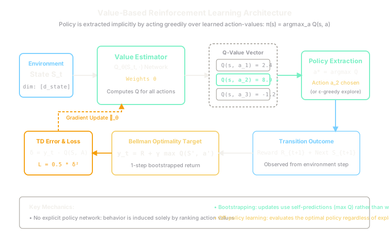
Value-based reinforcement learning evaluates action values and derives an optimal policy by greedily selecting the maximum predicted future return.

Why Does This Exist?

In sequential decision-making, choosing an action based solely on immediate rewards is short-sighted: an action that yields +1 right now might trap the agent in an inescapable failure state three steps later. Conversely, attempting to learn a policy directly by trial-and-error over entire trajectories requires collecting complete episodes before knowing whether a decision was sound. In high-dimensional environments with long horizons, this leads to crippling variance.

Value-based methods solve this by shifting the learning target from "what action should I take?" to "how much cumulative discounted reward will I collect if I take action $a$ in state $s$ ?". By learning an action-value function $Q(s, a)$ , the agent bypasses the need for an explicit parameterized policy network. The policy is induced for free by acting greedily with respect to the learned values: $\pi(s) = \arg\max_a Q(s, a)$ .

This paradigm anchors algorithms like tabular Q-learning, SARSA, and Deep Q-Networks (DQN). Before diving into specific update algorithms, understanding the value-based formulation reveals how dynamic programming transforms distant future objectives into tractable, step-by-step local updates.

Think of It Like This

A chess board evaluator instead of memorizing opening books

Imagine teaching someone to play chess. One approach is to hand them an encyclopedia of every conceivable move sequence and tell them which move to memorize for each board state—an explicit policy. For complex games, this book is infinitely large.

A value-based approach does something entirely different: it teaches the player to evaluate board positions. If the player learns that having a queen in the center with king safety is worth +9.2 points, while losing a rook is worth -5.0 points, they do not need a memorized rulebook for every board configuration. At any turn, they look at all legal moves, calculate the resulting position's value score, and pick the move that yields the highest score. The decision rule is simple arithmetic because the value function has already compressed thousands of future possibilities into a single numeric score.

How It Actually Works

Dynamic Programming and Bellman Optimality

Value-based methods operate on Markov Decision Processes formalized by the tuple $(\mathcal{S}, \mathcal{A}, \mathcal{P}, \mathcal{R}, \gamma)$ . Rather than parameterizing a policy $\pi_\theta(a|s)$ , value-based architectures parameterize an action-value function $Q_\theta(s, a)$ .

The optimal action-value function $Q^*(s, a)$ satisfies the Bellman Optimality Equation:

Q^*(s, a) = \mathcal{R}(s, a) + \gamma \sum_{s' \in \mathcal{S}} \mathcal{P}(s' \mid s, a) \max_{a' \in \mathcal{A}} Q^*(s', a')

Where:

$s \in \mathcal{S}$ is the current state vector of dimension $[d_{\text{state}}]$ .
$a \in \mathcal{A}$ is a discrete action from an action set of size $|\mathcal{A}|$ .
$\mathcal{R}(s, a)$ is the expected immediate scalar reward.
$\gamma \in [0, 1)$ is the discount factor ensuring convergence over infinite horizons.
$s'$ is the next state drawn from transition probability $\mathcal{P}(s' \mid s, a)$ .
$\max_{a'} Q^*(s', a')$ enforces the assumption that future actions will be chosen optimally.

In model-free settings where transition probabilities $\mathcal{P}$ are unknown, algorithms collect transition tuples $(S_t, A_t, R_{t+1}, S_{t+1})$ and construct a bootstrapped target:

y_t = R_{t+1} + \gamma \max_{a'} Q(S_{t+1}, a')

The learning objective minimizes the mean squared temporal difference (TD) error:

\mathcal{L}(\theta) = \mathbb{E}\left[ \left( y_t - Q_\theta(S_t, A_t) \right)^2 \right]

Differentiating with respect to parameter vector $\theta$ yields the semi-gradient update:

\theta \leftarrow \theta + \alpha \left( R_{t+1} + \gamma \max_{a'} Q_\theta(S_{t+1}, a') - Q_\theta(S_t, A_t) \right) \nabla_\theta Q_\theta(S_t, A_t)

The policy $\pi(a \mid s)$ is derived directly from the Q-function. To balance exploration during training, practitioners employ an $\epsilon$ -greedy mechanism:

\pi(a \mid s) = \begin{cases} 1 - \epsilon + \frac{\epsilon}{|\mathcal{A}|} & \text{if } a = \arg\max_{a'} Q(s, a') \\ \frac{\epsilon}{|\mathcal{A}|} & \text{otherwise} \end{cases}

Worked Example

Consider an agent in state $S_0$ choosing between two actions: $A_1$ (safe path) and $A_2$ (risky shortcut). The discount factor is $\gamma = 0.9$ , the learning rate is $\alpha = 0.4$ , and the current estimated Q-values are:

Q(S_0, A_1) = 3.0, \quad Q(S_0, A_2) = 2.5

Action Execution: Following an $\epsilon$ -greedy roll, the agent explores action $A_2$ .
Environment Response: The environment transitions the agent to next state $S_1$ and returns immediate reward $R = 1.0$ .
Evaluating Next State: In state $S_1$ , the available actions have estimated values $Q(S_1, A_1) = 5.0$ and $Q(S_1, A_2) = 4.0$ .
Target Calculation: $\max_{a'} Q(S_1, a') = \max(5.0, 4.0) = 5.0$ $y = R + \gamma \max_{a'} Q(S_1, a') = 1.0 + 0.9 \times 5.0 = 1.0 + 4.5 = 5.5$
Temporal Difference Error: $\delta = y - Q(S_0, A_2) = 5.5 - 2.5 = 3.0$
Q-Value Update: $Q(S_0, A_2) \leftarrow Q(S_0, A_2) + \alpha \times \delta = 2.5 + 0.4 \times 3.0 = 2.5 + 1.2 = 3.7$

After this single transition, $Q(S_0, A_2)$ increased from $2.5$ to $3.7$ . In future greedy selections from $S_0$ , the agent now prefers $A_2$ over $A_1$ ( $3.7 > 3.0$ ).

Code

1from typing import Dict, List, Tuple2import numpy as np3
4def update_q_value(5    q_table: Dict[str, np.ndarray],6    state: str,7    action_idx: int,8    reward: float,9    next_state: str,10    gamma: float = 0.9,11    alpha: float = 0.4,12) -> float:13    """Updates Q(s, a) using the 1-step Bellman optimality target."""14    current_q = q_table[state][action_idx]15    max_next_q = float(np.max(q_table[next_state]))16    td_target = reward + gamma * max_next_q17    td_error = td_target - current_q18    q_table[state][action_idx] = current_q + alpha * td_error19    return td_error20
21# Initialize tabular Q values for two states, each with 2 discrete actions22q_values: Dict[str, np.ndarray] = {23    "S0": np.array([3.0, 2.5], dtype=np.float64),24    "S1": np.array([5.0, 4.0], dtype=np.float64),25}26
27# Step transition: S0, action index 1 (A2), reward 1.0, lands in S128error = update_q_value(29    q_table=q_values,30    state="S0",31    action_idx=1,32    reward=1.0,33    next_state="S1",34    gamma=0.9,35    alpha=0.4,36)37
38print(f"TD Error: {error:.2f}")39# -> TD Error: 3.0040
41print(f"Updated Q(S0): {q_values['S0'].tolist()}")42# -> Updated Q(S0): [3.0, 3.7]43
44greedy_action = int(np.argmax(q_values["S0"]))45print(f"Optimal Action for S0: A{greedy_action + 1}")46# -> Optimal Action for S0: A2

Watch Out For

The Maximization Bias Trap

In noisy environments, using $\max_{a'} Q(S', a')$ systematically overestimates expected returns because $\mathbb{E}[\max(X_1, X_2)] \ge \max(\mathbb{E}[X_1], \mathbb{E}[X_2])$ by Jensen's inequality. If the estimated values of multiple suboptimal actions fluctuate around zero due to sampling variance or neural network approximation error, the $\max$ operator repeatedly grabs the positive noise spike, leading the agent to hallucinate high value in dead-end states.

To prevent explosive value overestimation in deep networks, implement Double Q-learning or Double DQN. Decouple action selection from action evaluation: use the online network to select the best action index $a^* = \arg\max_a Q_\theta(S', a)$ , but evaluate that action's value using a separate target network $Q_{\theta^-}(S', a^*)$ .

The Quick Version

Value-based methods replace explicit policy networks with an action-value function $Q(s, a)$ , extracting decisions greedily via $\arg\max_a Q(s, a)$ .
Learning is driven by the Bellman Optimality Equation, bootstrapping current estimates against a 1-step target: $R + \gamma \max_{a'} Q(s', a')$ .
Because they evaluate optimal actions off-policy, value-based methods are highly sample-efficient but require mitigation strategies like Double Q-learning to control maximization bias.