The REINFORCE Algorithm

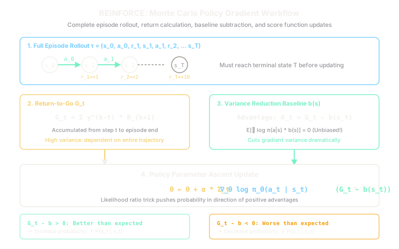
REINFORCE updates a neural network policy by waiting for complete episodes, increasing the probability of actions that produced high returns and penalizing actions that led to low returns.

The REINFORCE workflow: sampling full episode trajectories, computing returns-to-go, subtracting a baseline, and scaling log-probability policy gradients.

Why Does This Exist?

In many real-world control tasks, such as robotic arm manipulation or drone attitude stabilization, the action space is continuous (torque voltages, thrust vectors). Value-based methods struggle here: to act greedily, they must solve $\arg\max_a Q(s, a)$ at every timestep, which requires expensive continuous optimization inside the inner simulation loop. Furthermore, value-based methods cannot naturally learn stochastic policies, which are required in games of imperfect information or under state aliasing.

The REINFORCE algorithm (Williams, 1992) pioneered the policy gradient revolution. Instead of evaluating state-action values and deriving a policy indirectly, REINFORCE parameterizes the policy directly as $\pi_\theta(a \mid s)$ —typically outputting the mean and variance of a Gaussian distribution or logits of a categorical distribution.

Crucially, REINFORCE answers a fundamental question: how can you differentiate an objective function that depends on environment transitions when you do not know the environment's transition dynamics $\mathcal{P}(s' \mid s, a)$ ? By utilizing the log-derivative trick, REINFORCE converts the gradient of expected performance into an expectation of gradients, allowing agents to optimize policies via empirical Monte Carlo rollouts.

Think of It Like This

A basketball coach reviewing full game tape at the buzzer

Imagine a basketball coach who is not allowed to interrupt the game to give tactical corrections mid-play. Instead, the coach watches the entire 48-minute game from the stands without interfering, letting the players experiment with different passes and shots.

After the buzzer sounds and the final scoreboard confirms whether the team won or lost by 20 points, the coach sits down with the full game tape. For every shot taken in the fourth quarter, if the sequence ended in a scoring rally, the coach tells the player: "Do that exact dribble-drive move more often next time." If a sequence yielded turnovers and opponent fast-breaks, the coach says: "Reduce the frequency of that risky bounce pass."

Because the feedback is based on the entire completed game, credit is noisy—a brilliant pass in the first quarter might get dragged down by poor defense in the fourth. But across hundreds of games, the moves that systematically lead to high scores are reinforced, while moves that consistently lead to losses are suppressed.

How It Actually Works

Likelihood Ratio and Baseline Subtraction

Let a trajectory $\tau = (s_0, a_0, r_1, s_1, a_1, \dots, s_T)$ be sampled by following policy $\pi_\theta$ . The expected return objective is:

J(\theta) = \mathbb{E}_{\tau \sim \pi_\theta}[R(\tau)] = \int P(\tau; \theta) R(\tau) \, d\tau

The probability of a trajectory factors into initial state distribution, policy actions, and unknown environment transition probabilities:

P(\tau; \theta) = \rho_0(s_0) \prod_{t=0}^{T-1} \pi_\theta(a_t \mid s_t) \mathcal{P}(s_{t+1} \mid s_t, a_t)

Taking the gradient $\nabla_\theta J(\theta)$ directly is impossible because $\mathcal{P}$ is unknown. Applying the likelihood ratio trick ( $\nabla_\theta P(\tau) = P(\tau) \nabla_\theta \log P(\tau)$ ) eliminates the environment dynamics:

\nabla_\theta \log P(\tau; \theta) = \sum_{t=0}^{T-1} \nabla_\theta \log \pi_\theta(a_t \mid s_t)

This yields the Policy Gradient Theorem:

\nabla_\theta J(\theta) = \mathbb{E}_{\tau \sim \pi_\theta} \left[ \sum_{t=0}^{T-1} \nabla_\theta \log \pi_\theta(a_t \mid s_t) G_t \right]

Where $G_t$ is the return-to-go from step $t$ :

G_t = \sum_{k=t}^{T-1} \gamma^{k-t} R_{k+1}

Because future actions cannot influence past rewards, causality dictates replacing total trajectory return $R(\tau)$ with $G_t$ , drastically reducing gradient variance.

Baseline Variance Reduction

To further reduce variance without introducing bias, a state-dependent baseline $b(s_t)$ is subtracted from $G_t$ . The update becomes:

\theta \leftarrow \theta + \alpha \sum_{t=0}^{T-1} \nabla_\theta \log \pi_\theta(a_t \mid s_t) \left( G_t - b(s_t) \right)

The baseline does not introduce bias because:

\mathbb{E}_{a_t \sim \pi_\theta} \left[ \nabla_\theta \log \pi_\theta(a_t \mid s_t) b(s_t) \right] = b(s_t) \sum_{a} \pi_\theta(a \mid s_t) \frac{\nabla_\theta \pi_\theta(a \mid s_t)}{\pi_\theta(a \mid s_t)} = b(s_t) \nabla_\theta (1) = 0

Worked Example

Consider a 2-step episode in an environment with two discrete actions ( $a_1, a_2$ ) parameterized by a single policy weight $\theta \in \mathbb{R}$ . The policy uses a softmax distribution where logit for $a_1$ is $\theta$ and logit for $a_2$ is $0$ :

\pi_\theta(a_1 \mid s) = \frac{e^\theta}{e^\theta + 1} = \sigma(\theta), \quad \pi_\theta(a_2 \mid s) = 1 - \sigma(\theta)

The gradient with respect to $\theta$ is:

If $a_1$ is chosen: $\nabla_\theta \log \pi_\theta(a_1) = 1 - \sigma(\theta)$
If $a_2$ is chosen: $\nabla_\theta \log \pi_\theta(a_2) = -\sigma(\theta)$

Let initial weight $\theta = 0.0$ , so $\sigma(0.0) = 0.5$ ( $\pi(a_1) = 0.5, \pi(a_2) = 0.5$ ). Discount factor $\gamma = 1.0$ , learning rate $\alpha = 0.1$ , and constant baseline $b = 5.0$ .

Sampled Episode Rollout:

Step 0 ( $s_0$ ): Agent samples $a_1$ . Receives reward $r_1 = 2.0$ .
Step 1 ( $s_1$ ): Agent samples $a_2$ . Receives reward $r_2 = 8.0$ . Episode terminates ( $T=2$ ).

Step-by-Step Computations:

Returns-to-go:
$G_1 = r_2 = 8.0$ $G_0 = r_1 + \gamma G_1 = 2.0 + 8.0 = 10.0$
Advantage with Baseline:
$A_0 = G_0 - b = 10.0 - 5.0 = +5.0$ $A_1 = G_1 - b = 8.0 - 5.0 = +3.0$
Log-Probability Gradients:
- At $t=0$ , action was $a_1$ : $\nabla_\theta \log \pi(a_1) = 1 - 0.5 = +0.5$
- At $t=1$ , action was $a_2$ : $\nabla_\theta \log \pi(a_2) = -0.5$
Total Policy Gradient:
$\nabla_\theta J = (\nabla_\theta \log \pi(a_0) \cdot A_0) + (\nabla_\theta \log \pi(a_1) \cdot A_1)$ $\nabla_\theta J = (0.5 \times 5.0) + (-0.5 \times 3.0) = 2.5 - 1.5 = +1.0$
Parameter Update:
$\theta \leftarrow \theta + \alpha \nabla_\theta J = 0.0 + 0.1 \times 1.0 = 0.1$

New probability for $a_1$ : $\sigma(0.1) = \frac{e^{0.1}}{e^{0.1} + 1} \approx 0.525$ . The probability of taking action $a_1$ increased because its advantage was strongly positive.

Code

1from typing import List, Tuple2import numpy as np3
4def reinforce_update(5    theta: float,6    actions: List[int],7    rewards: List[float],8    gamma: float = 1.0,9    alpha: float = 0.1,10    baseline: float = 5.0,11) -> Tuple[float, List[float]]:12    """Executes a Monte Carlo REINFORCE parameter update over one episode."""13    # Compute returns-to-go G_t backward from terminal step14    returns: List[float] = [0.0] * len(rewards)15    g = 0.016    for t in reversed(range(len(rewards))):17        g = rewards[t] + gamma * g18        returns[t] = g19
20    # Softmax probability for action 0: p = 1 / (1 + exp(-theta))21    prob_a1 = 1.0 / (1.0 + np.exp(-theta))22    23    total_grad = 0.024    for t, action in enumerate(actions):25        advantage = returns[t] - baseline26        # Gradient of log pi: (1 - prob) if action 0, else -prob27        grad_log = (1.0 - prob_a1) if action == 0 else (-prob_a1)28        total_grad += grad_log * advantage29
30    updated_theta = theta + alpha * total_grad31    return updated_theta, returns32
33# Episode: action 0 (a1) then action 1 (a2), rewards 2.0 and 8.034init_theta = 0.035new_theta, returns_computed = reinforce_update(36    theta=init_theta,37    actions=[0, 1],38    rewards=[2.0, 8.0],39    gamma=1.0,40    alpha=0.1,41    baseline=5.0,42)43
44print(f"Returns G_t: {returns_computed}")45# -> Returns G_t: [10.0, 8.0]46
47print(f"Updated Theta: {new_theta:.2f}")48# -> Updated Theta: 0.1049
50new_prob = 1.0 / (1.0 + np.exp(-new_theta))51print(f"Updated P(a1): {new_prob:.4f}")52# -> Updated P(a1): 0.5250

Watch Out For

The Monte Carlo Variance Explosion

Because REINFORCE computes full episodic returns $G_t$ by summing across all subsequent timesteps, the variance of the gradient estimator compounds exponentially with episode horizon $T$ . A single stochastic transition or exploratory action near the end of the episode introduces noise into the gradient of every preceding action in that episode, causing training to stall or destabilize.

Always implement reward-to-go instead of total trajectory return, normalize advantages across batch rollouts ( $\frac{A - \mu_A}{\sigma_A + 10^{-8}}$ ), and subtract a learned state-value baseline $V_\phi(s)$ . If episode horizons exceed a few hundred steps, transition from pure Monte Carlo REINFORCE to an Actor-Critic architecture that bootstraps after $n$ steps.

The Quick Version

REINFORCE uses the log-derivative likelihood ratio trick to optimize parameterized policies without knowing environment transition dynamics.
Updates occur strictly at the end of complete episodes using Monte Carlo returns-to-go: $G_t = \sum_{k=t}^T \gamma^{k-t} R_{k+1}$ .
Subtracting an unbiased baseline $b(s_t)$ from $G_t$ preserves the expected gradient while dramatically reducing sampling variance.