Diffusion Models for Image Generation

Treat Pixels As A Joint Vector

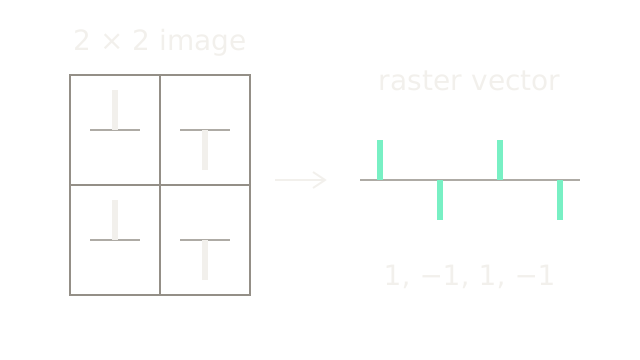
Diffusion image generation learns to reverse a known corruption process. Training pairs noisy images with sampled noise; generation repeatedly uses a learned denoiser to transform fresh noise into a new image. It does not simply retrieve the original photograph hidden inside a random sample.

Use a synthetic two-by-two grayscale image x0=[1,−1;1,−1], flattened in raster order to [1,−1,1,−1]. Each stem is one normalized pixel value relative to its horizontal zero baseline. Positive points up and negative down; these are values, not spatial heights in a photographed scene. The general diffusion visual covers distributions and guidance. Here we inspect image coordinates and distinguish training from sampling.

Add A Known Noise Draw

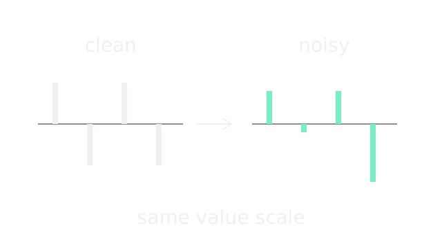
Let cumulative retention be ᾱt=0.64. The noisy sample follows

$$x_t=\sqrt{\bar\alpha_t}\,x_0+\sqrt{1-\bar\alpha_t}\,\epsilon.$$

Choose the illustrative noise vector ε=[0,1,0,−1]. Then xt=0.8x0+0.6ε=[0.8,−0.2,0.8,−1.4]. The two panels use sixty drawing units per value unit. The fourth coordinate becomes more negative: adding noise does not mean monotonically shrinking every pixel. Noisy coordinates can leave the clean normalized range. This chosen vector illustrates an aggregate Gaussian draw, not a claim that noise takes only three discrete values.

Multiply The Retention Schedule

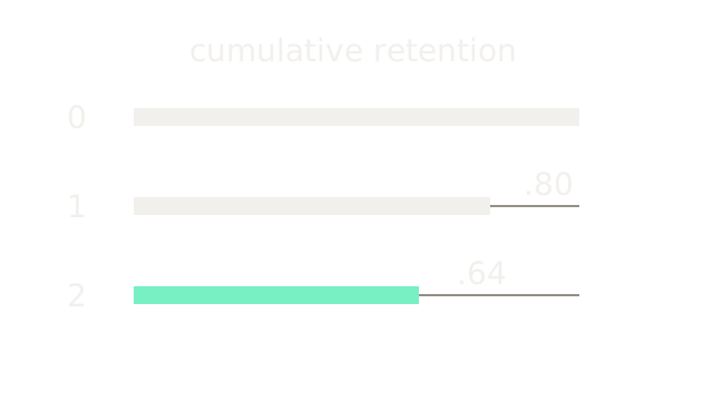
Per-step retention is αt=1−βt, where βt is the added noise variance. Cumulative retention is the product ᾱt=∏s≤t αs. Two illustrative steps with α equal to 0.8 give cumulative values 1,0.8,0.64. Bars encode these cumulative coefficients at four hundred drawing units per unit. The signal amplitude coefficients are their square roots, not these bar lengths: 1,√0.8,0.8. Our two large steps make arithmetic visible; they are not a recommended image-training schedule.

Construct The Training Pair

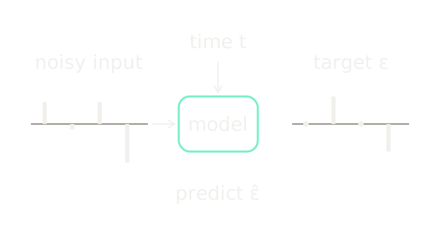
Sample a clean training image, a timestep t, and noise ε. Construct xt using the forward rule. The network receives (xt,t) and predicts ε̂; the sampled ε is the supervision target, not an input shortcut. The drawing keeps that target to the right with no input arrow. Pixel stems use forty drawing units per value unit here, a deliberate zoom out from the previous value plot. Time conditioning tells the shared model which corruption level it should interpret.

Penalize Noise Prediction Errors

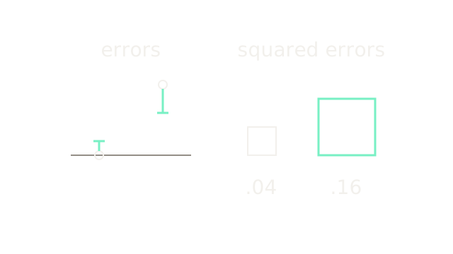
Zoom to two coordinates with target noise [0,1] and predicted noise [0.2,0.6]. Errors are 0.2 and −0.4; squared errors are 0.04 and 0.16. Their mean is 0.10. On the left circles are targets and short ticks predictions, at one hundred drawing units per noise unit. On the right, square sides are forty and eighty units, making areas proportional to squared error with ratio four. The DDPM paper's simplified objective uses a squared noise-prediction error; sums or means over coordinates differ by a scale factor.

Estimate The Clean Image

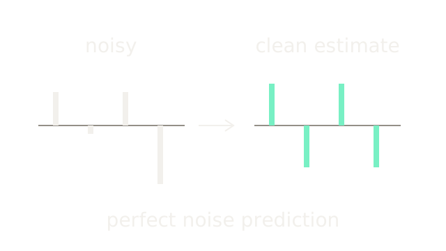
Rearrange the forward relation:

$$\hat x_0=\frac{x_t-\sqrt{1-\bar\alpha_t}\,\hat\epsilon}{\sqrt{\bar\alpha_t}}.$$

With the exact illustrative ε from beat 2, this becomes (xt−0.6ε)/0.8=[1,−1,1,−1]. Both panels return to sixty drawing units per value unit. This exact result is an arithmetic check using privileged knowledge of the chosen noise. A trained predictor need not recover that particular draw perfectly. Most importantly, this clean estimate is not automatically the next noisy sampling state xt−1.

Compute A Reverse Mean

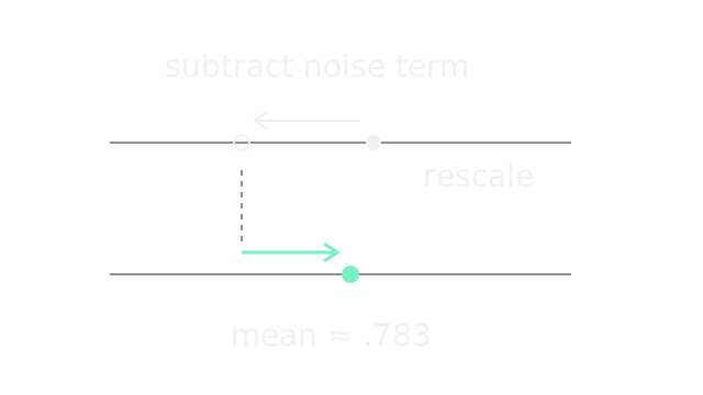
For the noise-prediction parameterization, one reverse mean is

$$\mu_\theta(x_t,t)=\frac{1}{\sqrt{\alpha_t}} \left(x_t-\frac{\beta_t}{\sqrt{1-\bar\alpha_t}}\hat\epsilon\right).$$

Use a separate one-coordinate model-output fixture: xt=0.8, αt=0.8, βt=0.2, ᾱt=0.64, and ε̂=0.3. Subtract (0.2/0.6)×0.3=0.1 to get 0.7, then divide by √0.8 to get μ≈0.782623792. The cropped number lines share a scale of twelve hundred drawing units per value unit; row separation keeps subtraction and rescaling distinct. These are reverse-mean coefficients, different from those in the clean estimate.

Sample Around That Mean

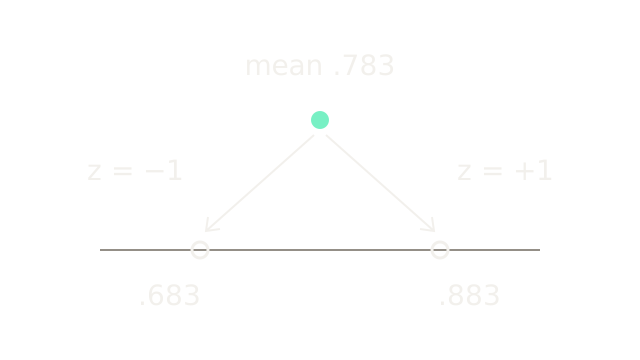
A stochastic step uses xt−1=μθ+σt z, with fresh standard Gaussian z. Keep the preceding mean and choose illustrative σt=0.1. Draws z=−1 and z=+1 produce 0.682623792 and 0.882623792. Branches show two example outcomes, not two equiprobable point masses; the actual Gaussian is continuous. This chosen standard deviation illustrates the operation rather than a particular trained model's variance schedule. DDPM's final sampling step omits the fresh noise term.

Repeat The Denoising Chain

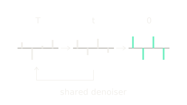
Start generation from a fresh sample approximately distributed as standard Gaussian noise, then repeatedly predict noise, compute an update, and advance to a lower noise level. The same network parameters serve successive timesteps; t changes at each call. The lower loop denotes that reuse rather than forward corruption.

The three pictured vectors are illustrative states [0.5,−1,0.2,0.7], [0.7,−0.6,0.8,−0.4], and [1,−1,1,−1] at forty drawing units per value unit. They show changing image structure, not outputs from a trained network or a numerically simulated DDPM trajectory. Repeated evaluation buys a gradual generative process at the cost of multiple denoiser calls. Other samplers change that trade-off.

Where It Breaks

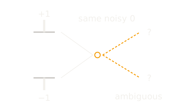
Consider one coordinate at ᾱt=0.64. Clean value +1 with noise −4/3 gives 0.8×1+0.6×(−4/3)=0. Clean value −1 with noise +4/3 also gives zero. The solid paths merge; dashed reverse paths ask which original produced it. This is a concrete many-to-one ambiguity, not a claim that exact points have nonzero Gaussian probability.

At sampling time the particular training noise target is unavailable. A denoiser learns statistical structure, so plausible detail can be generated without proving historical truth or restoring the original pixels. Do not use visual plausibility as evidence that an image restoration recovered a fact. Conditioning can restrict possible outputs, but cannot manufacture missing evidence.

The Quick Version

• An image is a joint vector of pixel values.
• Forward corruption attenuates signal and adds Gaussian noise.
• Cumulative retention multiplies per-step coefficients.
• Training knows the sampled noise used to corrupt each image.
• Squared prediction errors provide a denoising training signal.
• A clean estimate differs from the next noisy state.
• The reverse mean uses timestep-dependent subtraction and rescaling.
• Stochastic sampling adds controlled variation around that mean.
• Generation repeatedly reuses a time-conditioned denoiser.
• A plausible generated image cannot prove a unique original.