Vision Transformers and Patch Attention

Cut The Image Into Patches

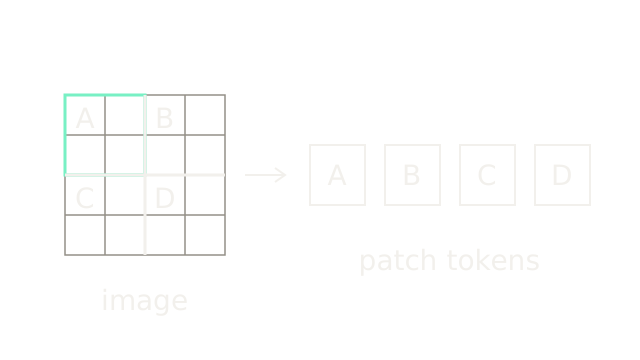
A Vision Transformer (ViT) represents image patches as vectors, lets them exchange information through attention, and uses the resulting representation for a task such as classification. A patch is a block of pixels; a token is its vector representation.

The toy grayscale image is four-by-four pixels. Two-by-two patches produce four tokens A–D in raster order. In general an H-by-W image with square patches of side P has N=HW/P² patches when both dimensions divide evenly. Each flattened RGB patch has P²×3 values. The ViT method defines the patch projection and encoder; this page uses smaller synthetic vectors to inspect the operations.

Project Pixel Values

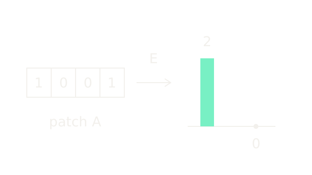
Flatten patch A to [1,0,0,1]. Choose a toy projection E with rows (1,0), (0,1), (0,−1), (1,0). Multiplying gives embedding (2,0): the first coordinate adds diagonal pixels, while the second subtracts the off-diagonal ones. Bars use seventy drawing units per embedding unit. This is not average pooling, and E is learned in a real model. Compressing to fewer coordinates can discard information.

Add Position Information

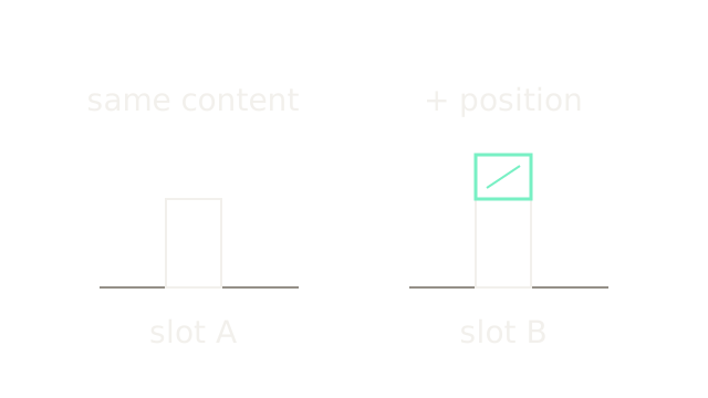
Two patches with the same content vector otherwise start identically. Illustrate one coordinate with content 2 and position contributions 0 at slot A and 1 at slot B: the inputs become 2 and 3. Unfilled bars show equal content; the hatched cap shows the added positional component, at forty drawing units per coordinate unit. Actual learned position embeddings are vectors, not literal image coordinates. Their addition lets attention learn spatial relationships.

Compare Queries With Keys

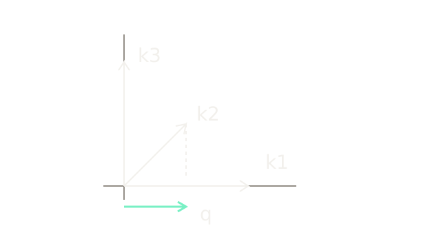
Each token is projected into query, key and value vectors. A query asks which token information should contribute. For synthetic q=(1,0) and keys (2,0), (1,1), (0,2), raw dot products are 2,1,0. Horizontal projections make those scores visible at ninety drawing units per component. The mint q arrow is translated below the shared origin to keep it readable. For key dimension two, scaled logits would be [2,1,0]/√2. Embedding axes have no assigned human meaning.

Normalize One Attention Row

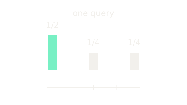
For easy exact arithmetic, switch to a separate three-key row whose already-scaled logits are [ln(2),0,0]. Exponentials are [2,1,1]; dividing by their sum 4 gives weights [0.5,0.25,0.25]. This is not the normalized result of the previous beat's logits. Bar heights share a probability scale and the strip partitions unit total mass. Softmax emphasizes the highest score without selecting only that key.

Blend The Value Vectors

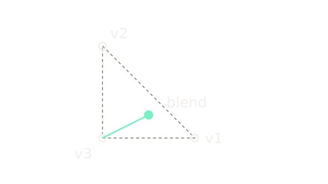
Retain those exact weights and use values v1=(2,0), v2=(0,2), v3=(0,0). Their weighted sum is 0.5v1+0.25v2+0.25v3=(1,0.5), the mint point inside the value triangle. Axes are value coordinates at ninety drawing units per unit; this is not a location in the image. Multiple heads form separate blends before concatenation and an output projection. See attention mechanics for that broader mechanism.

Connect Distant Patches

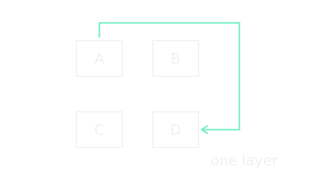
Return to the four spatial patches. The routed link shows that A and diagonal patch D can interact without first traversing B or C. The route is a schematic dependency, not physical travel or a measured attention weight. Full attention permits all token pairs, including self-pairs; one path is drawn to isolate nonlocal access. Access does not guarantee a large weight or successful object reasoning.

Add The Residual Update

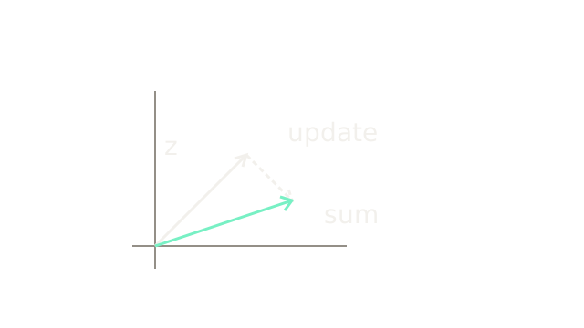
For a synthetic token z=(1,1) and attention-block update (0.5,−0.5), residual addition yields (1.5,0.5). The dashed update starts at z's endpoint; the mint vector reaches the sum from the common origin. This is vector addition at one hundred drawing units per component, with vertical coordinates inverted on the canvas. In ViT, normalization precedes attention; another normalized, tokenwise MLP block and residual addition follow. Attention mixes across tokens, while that MLP transforms each token independently with shared parameters.

Read The Class Token

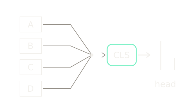
The original classification design prepends a learned CLS token, making five tokens for our four-patch image. Across encoder layers it can aggregate patch evidence. Its final normalized state feeds a classification head. The junction summarizes aggregation rather than a fixed equal average; the two output strokes indicate schematic class scores, with no numerical probability claim. The patch tokens also update during the encoder. A class token is learned task state, not a fifth image crop.

Where It Breaks

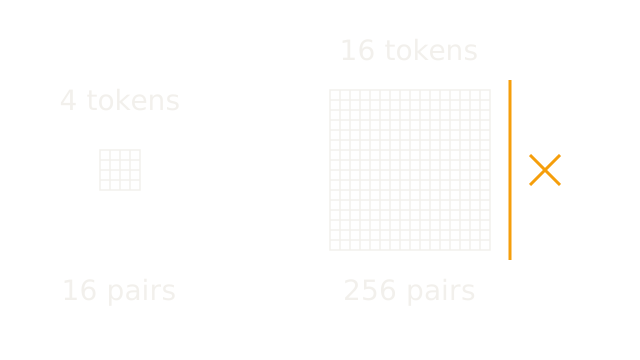
Halve patch side length on the same image: four patches become sixteen. Excluding CLS to isolate patch pairs, one attention head's score grid grows from 4²=16 to 16²=256 entries. Equal cell sizes make the sixteenfold growth visible. Including CLS gives 25 versus 289 entries. The amber boundary marks a finite capacity limit, not a measured device specification.

This count is pairwise work and, for a materialized attention matrix, storage; it is not total model runtime. Memory-efficient attention can avoid storing the complete matrix while retaining pair computations. Coarser patches reduce cost but limit spatial granularity. When local structure and small training sets dominate, convolutional image models offer a stronger built-in locality bias; global access alone is no guarantee of better predictions.

The Quick Version

• Nonoverlapping image patches become ordered tokens.
• Learned projection combines individual pixel values into embedding coordinates.
• Position embeddings distinguish identical content at different slots.
• Query-key dot products determine compatibility scores.
• Softmax creates normalized weights for each query.
• Attention blends values into a new token representation.
• Global attention permits distant patches to interact directly.
• Residual additions retain the previous representation alongside updates.
• A class token gathers evidence for classification.
• Finer patches can overwhelm global attention's pairwise budget.