Dynamics and Impedance Control

Dynamics relates forces and torques to a robot's acceleration. Impedance control shapes how the robot moves when something pushes it, using a chosen relationship between displacement, velocity and force. It can let a tool yield under contact while still pulling it toward a reference; achieving that behavior depends on the robot's actual dynamics, sensing and actuator limits.

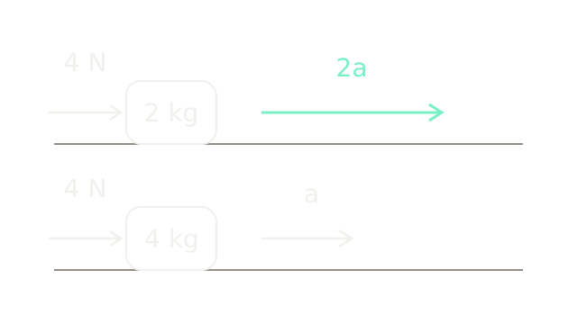
Imagine a robot tool constrained to a horizontal rail. Position tells us where it is; velocity tells us how fast position changes; acceleration tells us how fast velocity changes. Both pictured tools receive a four-newton motor force. Ignoring friction and other horizontal forces, Newton's law gives $a=F/m$: the 2 kg tool accelerates at $4/2=2$ m/s², while the 4 kg tool accelerates at $4/4=1$ m/s². The acceleration arrows have a two-to-one length ratio. Equal-size blocks are symbols, not a volume or density comparison.

A force command therefore does not directly select a position. The resulting motion also depends on mass, the initial velocity and other forces. Throughout the main rail example, positive motion and force point right. The mass is 2 kg and gravity has no component along the rail. A separate vertical example below introduces gravity explicitly.

Where does joint torque go?

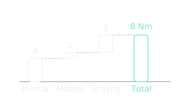
A rotating robot joint uses torque, measured in newton metres, rather than a linear force. The waterfall shows a synthetic snapshot: four newton metres for the desired acceleration, one for velocity-dependent effects, and three for gravity. Twenty pixels represent one newton metre in every bar, so the increments add to an eight-newton-metre request. These values illustrate the accounting; they are not measured data from a particular arm.

For a fully actuated arm, one common convention writes the dynamics as

$M(q)\ddot q+c(q,\dot q)+g(q)=\tau+J(q)^T F_{ext}.$

Here $q$ contains joint positions, $\dot q$ their velocities and $\ddot q$ their accelerations. The mass matrix $M$ describes inertia, including coupling between joints. The vector $c$ contains Coriolis and centrifugal effects; $g$ is the torque required to balance gravity; $\tau$ is applied motor torque. The Jacobian $J$ maps joint velocity to tool velocity, and $F_{ext}$ is the environment's force on the tool, expressed in the matching frame. Friction is omitted here and may require its own model.

In free space, inverse dynamics evaluates the left side for a desired acceleration to estimate the needed torque. Feedback still corrects tracking error and model mismatch. Treating each joint as an isolated mass can miss that moving one link changes the loading of another.

Support weight before correcting error

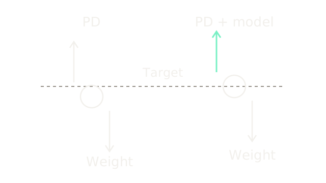
This separate vertical fixture uses a 2 kg point load and a deliberately rounded $g=10$ m/s², giving a downward weight of 20 N. The dashed line is its desired height. With a position spring of $K_p=1000$ N/m and no integral action, a stationary PD controller needs a downward offset of $20/1000=0.02$ m to request the supporting 20 N. The left circle is therefore two centimetres below target, shown at 1000 pixels per metre. D contributes nothing at rest.

Adding an accurate gravity estimate supplies those 20 N before position feedback contributes anything. The right circle can sit at the target with zero position error. Equal upward and downward arrow lengths show static balance; each arrow uses four pixels per newton. This compares equilibria, not settling trajectories.

Model-based support lets the feedback gains serve the desired contact behavior instead of merely fighting weight. It does not eliminate uncertainty: an unmodeled payload or inaccurate gravity estimate leaves a residual load. Continue with feedback control and PID for error, integral memory and saturation.

Give position error a spring

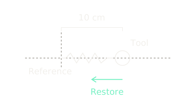
Return to the horizontal 2 kg tool. Choose a fixed reference $x_d=0$ and define displacement $\delta=x-x_d$. A virtual spring commands

$F_{spring}=-k\delta.$

With stiffness $k=100$ N/m and the tool displaced $\delta=+0.10$ m, the controller requests $-10$ N, toward the reference. The 200-pixel gap represents ten centimetres at 2000 pixels per metre; the restoring arrow uses ten pixels per newton. The drawn coil is a symbol for a force law implemented by the controller. No physical spring needs to connect these points.

Stiffness measures how much force changes per unit displacement. Increasing it reduces static yielding under a given load, but also increases the requested force for the same position error. A reference accidentally placed inside a rigid surface can therefore create a substantial contact request. A compliant controller still resists displacement; its resistance is deliberately specified.

Oppose motion with a damper

A spring stores energy and can return it, allowing oscillation. A virtual damper adds a force proportional to velocity relative to the reference:

$F_{damper}=-b(\dot x-\dot x_d).$

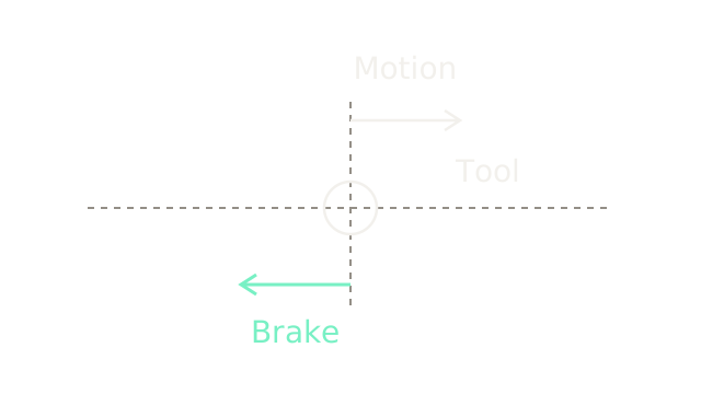
For our fixed reference, $\dot x_d=0$. Choose $b=20$ N·s/m. A rightward velocity of $+0.20$ m/s produces a leftward request of $-4$ N. The two arrows occupy different lanes because one is velocity and the other is force: the upper uses 500 pixels per m/s, the lower 25 pixels per newton. Compare their opposing directions, not the equality of their pixel lengths.

Damping vanishes at rest, regardless of position error. For the ideal one-dimensional system, the damping ratio is $\zeta=b/(2\sqrt{mk})$. With $m=2$, $k=100$ and $b=20$, it is approximately 0.707. Critical damping would require $b=2\sqrt{200}\approx28.28$ N·s/m for this particular model. A multidimensional robot has configuration-dependent inertia; copying this scalar value to every Cartesian axis does not establish critical damping.

Combine motion and contact forces

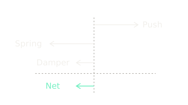
Suppose the environment pushes the tool right with $F_{ext}=+10$ N while the tool is already ten centimetres right of the reference and moving right at 0.20 m/s. The spring requests $-100(0.10)=-10$ N; the damper requests $-20(0.20)=-4$ N. All four arrows use fifteen pixels per newton, so the opposing ten-newton arrows cancel and the net arrow points left:

$m\ddot\delta=F_{ext}-b\dot\delta-k\delta=10-4-10=-4\text{ N}.$

Dividing by the 2 kg mass gives $\ddot\delta=-2$ m/s². This is an instantaneous force balance. The tool is still moving right, but its rightward velocity is decreasing. Acceleration and velocity need not point the same way.

Rearranging gives the desired mass–spring–damper relationship:

$m\ddot\delta+b\dot\delta+k\delta=F_{ext}.$

This equation is the impedance: it specifies how external force relates to motion. Here the inertia remains the physical 2 kg mass. Full impedance controllers may also shape apparent inertia, requiring additional modeling and often force or acceleration information. A spring–damper torque law alone does not let us assign any apparent mass we want.

How far does contact move it?

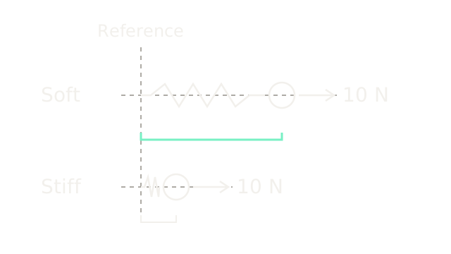
At a stationary equilibrium, velocity and acceleration are zero, leaving $k\delta=F_{ext}$. The upper tool has $k=100$ N/m and settles at $\delta=10/100=0.10$ m under a constant 10 N external push. The lower tool has $k=400$ N/m and settles at $10/400=0.025$ m. The common position scale is 2000 pixels per metre, giving offsets of 200 and 50 pixels. Equal external arrows show the same ten-newton load in both cases.

The soft tool moves four times farther. It does not exert less force at this equilibrium: both controllers balance the imposed 10 N. The advantage of lower stiffness appears under a given geometric error or uncertain contact location, where $F=k\delta$ gives a smaller force request. Greater compliance trades positioning precision under load for yielding.

This also separates impedance control from direct force regulation. Impedance establishes a force–motion relationship; the actual contact force emerges from that relationship and the environment. With a rigid wall at $x_w$, a stationary tool touching it has a spring request determined by $k(x_w-x_d)$. Choosing stiffness alone cannot guarantee an arbitrary force when the wall position is unknown. Admittance control takes the opposite interface direction: measured force drives a motion reference, often for a robot with an inner position loop.

Follow the energy during release

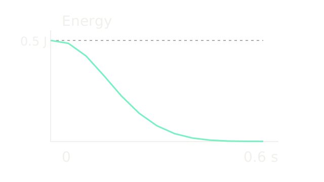
Now release the same horizontal system from a ten-centimetre displacement at rest, with no external push. This is a new initial condition, not the moving snapshot above. Its stored mechanical energy is

$E=\tfrac12m\dot\delta^2+\tfrac12k\delta^2.$

Initially $E=0+\tfrac12(100)(0.10)^2=0.5$ J. For $m=2$, $b=20$ and $k=100$, the exact displacement and velocity are

\dot\delta(t)=-e^{-5t}\sin(5t).$$ The plot connects exact energy samples every 0.05 seconds, using 700 pixels per second horizontally and 400 pixels per joule vertically. At 0.20 seconds, $\delta\approx0.05083$ m and $\dot\delta\approx-0.30956$ m/s give $E\approx0.22502$ J. At 0.60 seconds it is approximately 0.000942 J. Straight segments visualize those samples; they are not an integration algorithm. The useful invariant follows by differentiation: $$\dot E=\dot\delta(m\ddot\delta+k\delta) =F_{ext}\dot\delta-b\dot\delta^2.$$ Without external force, $\dot E=-b\dot\delta^2\le0$: damping removes energy while the ideal spring exchanges stored and kinetic energy. A moving reference can inject energy, and sampled control, delay or an inaccurate model can spoil this ideal argument. A positive damping gain in software is not, by itself, a proof that a physical robot interacting with any environment remains passive. ## Turn tool force into joint torque <AnimatedDiagram src="/diagrams/visuals/dynamics-and-impedance-control/09-task-force-to-torque.svg" title="A tool force maps to joint torque through its lever arm." /> For a robot arm, a desired tool force must become joint torques. The one-hinge example has a horizontal 0.5 m lever arm and a downward 10 N tool force. Its torque is $\tau_z=r_xF_y=0.5(-10)=-5$ Nm, clockwise. The arm uses 300 pixels per metre and the downward force uses ten pixels per newton; the curved arrow shows direction only. For several joints, virtual work gives $\tau_{task}=J^T F_{cmd}$. The transpose preserves power: $\tau_{task}^T\dot q=F_{cmd}^T(J\dot q)$. Use a wrench and Jacobian expressed at the same point and in the same frame. Adding model compensation then gives a common stiffness-control structure such as $$\tau=\hat g+J^T[K(x_d-x)+B(\dot x_d-\dot x)].$$ Here $K$ and $B$ are stiffness and damping matrices, and $\hat g$ estimates the gravity-balancing torque under our earlier sign convention. Additional Coriolis compensation or inertia shaping requires its own assumptions. The simple formula does not cancel the arm's full configuration-dependent dynamics. The [Jacobian visual](/visuals/physical-ai/jacobians-and-singularities) builds the velocity mapping and its singularity limits. ## Where it breaks <AnimatedDiagram src="/diagrams/visuals/dynamics-and-impedance-control/10-saturation-breaks-impedance.svg" title="Saturation breaks the requested spring behavior." /> Return to the horizontal rail, with stiffness 100 N/m, displacement $+0.20$ m and zero velocity. The spring asks for $-20$ N, shown dashed. Suppose the actuator can supply only $\pm12$ N. It applies $-12$ N instead. Under an external push of $+16$ N, the actual net force is $16-12=+4$ N, so the 2 kg tool accelerates **away** from the reference at $+2$ m/s². Every force arrow uses fifteen pixels per newton. The unconstrained spring model predicts an equilibrium at $16/100=0.16$ m. Reaching that equilibrium would require 16 N of restoring force, beyond the actuator's 12 N limit. With the stated constant load and no other resistance, no static equilibrium exists. Raising stiffness cannot create the missing actuator force. See [actuators, gearing and torque limits](/visuals/physical-ai/actuators-gearing-and-torque-limits) for the physical effort budget. Torque limits, delay, velocity-estimation noise, friction and uncertain payloads all separate requested behavior from realized behavior. High stiffness against a rigid environment can also demand fast, accurate control. Use direct force regulation when a specified contact force is the main objective and the hardware supports it; use impedance when the intended interaction is better expressed as yielding around a reference. Neither choice removes the need to check contact conditions and achievable effort. ## The Quick Version - Force sets acceleration through mass and other acting forces. - Robot dynamics includes inertia, velocity effects, gravity and external contact. - Gravity compensation can support weight without steady position error. - Virtual springs restore displacement toward a chosen reference. - Virtual dampers oppose velocity relative to that reference. - Impedance specifies a force–motion relationship, including dynamic effects. - Lower stiffness increases yielding under a fixed external load. - Ideal damping dissipates energy when the reference stays fixed. - Jacobian transpose maps compatible tool forces into joint torques. - Saturation can make the requested impedance physically unattainable. ## Sources [MIT's Manipulator Control notes](https://manipulation.csail.mit.edu/force.html) develop gravity compensation, joint stiffness control and Cartesian interaction dynamics. [Modern Robotics](https://hades.mech.northwestern.edu/images/b/b2/MR-2up.pdf), Chapters 5, 8 and 11, provides virtual work, manipulator dynamics and impedance control. [Franka's Cartesian impedance example](https://github.com/frankarobotics/libfranka/blob/main/examples/cartesian_impedance_control.cpp) implements a spring–damper law without inertia shaping. [The Franka interface documentation](https://support.franka.de/docs/libfranka.html) describes torque interfaces, filtering and command constraints. Numerical fixtures and the release calculation on this page are synthetic teaching examples, not robot operating recommendations or measured performance.