SLAM: Mapping While Localizing

SLAM estimates a robot's trajectory and its environment together. Motion measurements connect robot poses; observations connect those poses to landmarks or previously visited places. Because both are uncertain, new evidence can revise the map and past poses together.

The Kalman filter visual follows an uncertain position against a supplied observation model. Here the reference landmark itself becomes an unknown. We use small synthetic examples so that every change in the drawings can be checked, rather than presenting an optimizer as a box that produces a perfect map.

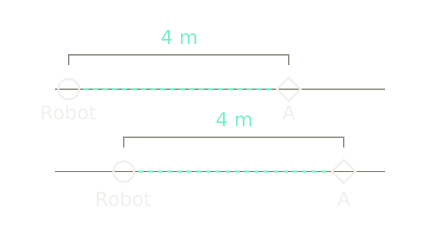
The circles are robot positions; diamonds are the same landmark A under two possible maps. In the upper row the robot is at 0 metres and A at 4. In the lower row they are at 1 and 5. Both predict the same relative separation, $A-x=4$ m. The 320-pixel brackets use 80 pixels per metre; vertical separation distinguishes hypotheses, not physical height.

An observation of something four metres ahead does not tell you the global coordinate of either endpoint. Add the same translation to both, and their difference stays unchanged. That ambiguity is a property of the available information, even with a perfectly accurate relative sensor.

Choose the map origin

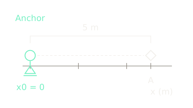
For the worked problem, choose the first robot position $x_0=0$ exactly. The triangular pin marks a coordinate anchor. It does not represent a GPS reading, a physical stop or an assertion that we know the robot's Earth coordinates.

Start a new synthetic dataset with an observation $z_0=5$ m ahead to A. Initializing the landmark at $A=5$ satisfies that observation, giving the 400-pixel bracket at the same 80-pixels-per-metre scale. It remains an estimate: later observations can move A. The anchor removes the translation ambiguity of this one-dimensional model; it does not make the other measurements exact. A real pose includes orientation, which this known-heading example deliberately leaves out.

Chain the motion estimates

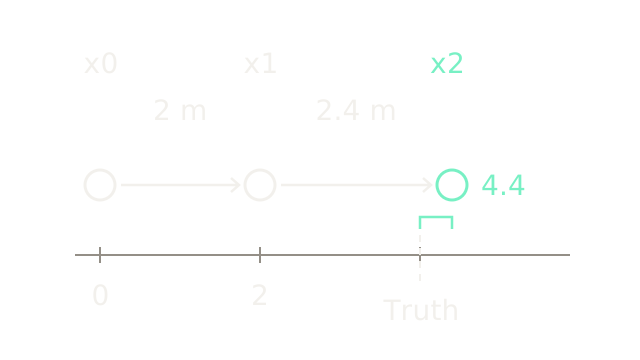
Suppose odometry reports successive forward increments $u_1=2$ m and $u_2=2.4$ m. Chaining them gives initial positions $x_1=2$ and $x_2=4.4$ m. Circle spacing is proportional to these increments at 80 pixels per metre. The dashed marker at 4 m is an illustrative ground-truth reference available to us, excluded from the estimator's inputs.

For the calculation below, assume each motion increment and each landmark observation has independent, zero-mean Gaussian noise with standard deviation $\sigma=0.2$ m, hence variance $\sigma^2=0.04$ m². The landmark is static, sensor calibration is already included, and all translations share a known axis. These assumptions define a linear teaching model, not a claim about a particular robot's sensors.

Compare the returning observation

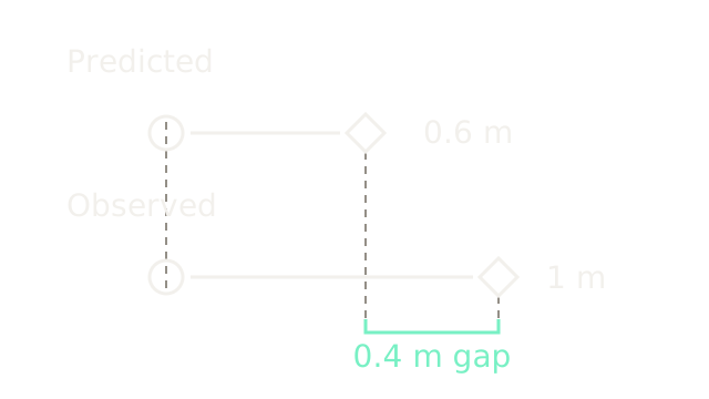
At the last pose, the sensor reports A one metre ahead: $z_2=1$ m. The initial map and odometry instead predict $A-x_2=5-4.4=0.6$ m. The two rows compare range, recentered on a common zero and zoomed to 300 pixels per metre. They are not two absolute landmark locations. Their 120-pixel endpoint difference represents 0.4 m.

Define a residual as predicted minus observed:

$r_{z_2}=A-x_2-z_2=5-4.4-1=-0.4\text{ m}.$

This disagreement could come from motion error, landmark error or observation noise. Assigning all of it to the robot would treat the current map as exact. SLAM allows the evidence to change both.

Is it the same landmark?

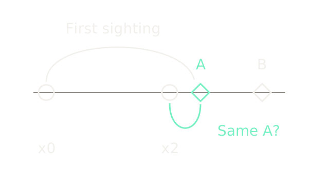
The arcs associate two sightings with A, while B remains a distinct landmark. Arc length has no numerical meaning; horizontal object positions use 60 pixels per metre. This identity illustration places the second robot at the observation-consistent candidate $x_2=4$ m, not at the final joint solution. A is at 5 and B at 7 m.

Data association decides which existing landmark, if any, generated an observation. Matching appearance, predicted geometry and uncertainty can supply evidence; a similar-looking object alone does not establish identity. A new landmark and a reobserved landmark lead to different estimation problems. The next two beats assume the association to A is correct and return to the original odometry initialization.

Connect the shared unknowns

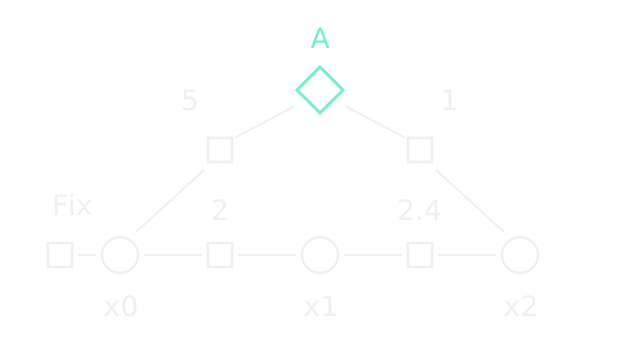
This is a schematic factor graph, so spacing no longer measures metres. Circles are robot positions, the diamond is A, and squares are constraints. The bottom factors carry motion measurements 2 and 2.4; the upper factors carry observations 5 and 1. The left square fixes $x_0$. Each observation square touches both the robot variable and the shared landmark variable it constrains. This follows the GTSAM landmark-SLAM construction.

With $x_0=0$, minimize the sum of squared residuals divided by their variances:

$$J(x_1,x_2,A)= \frac{(x_1-2)^2}{0.04} +\frac{(x_2-x_1-2.4)^2}{0.04} +\frac{(A-5)^2}{0.04} +\frac{(A-x_2-1)^2}{0.04}.$$

All four numerators have units m², so J is dimensionless. Equal denominators give equal weight here; a larger observation variance would reduce that term's influence. Independence is an explicit assumption: treating correlated evidence as separate independent factors can overstate information.

This map contains a point landmark, not walls, free space or a collision grid. SLAM representations differ; localization and mapping discusses that choice. An estimated landmark map alone is insufficient for checking a robot body's path through obstacles.

Revise map and trajectory together

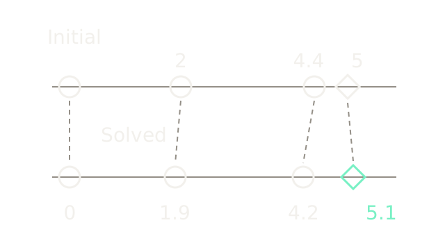
Both rows restore the shared 80-pixels-per-metre coordinate scale. Dashed guides track each variable across the update. The anchor stays fixed. The solution moves $x_1$ left by 0.1 m, $x_2$ left by 0.2 m, and A right by 0.1 m:

$x_1^*=1.9\text{ m},\qquad x_2^*=4.2\text{ m},\qquad A^*=5.1\text{ m}.$

Substitution gives residuals $(-0.1,-0.1,+0.1,-0.1)$ m in the equation's order. Initially they were $(0,0,0,-0.4)$ m. Thus J falls from $0.4^2/0.04=4$ to $4(0.1^2/0.04)=1$. The signs balance the normal equations: the derivative for $x_1$ subtracts the first two residuals, for $x_2$ subtracts the fourth from the second, and for A adds the third and fourth. All are zero at the stated solution.

This anchored linear quadratic has a unique minimum. Real poses and camera observations generally require nonlinear optimization and an initial estimate; the GTSAM optimization example demonstrates repeated linearization. Lower cost means better agreement with the assumed model and factors. It does not certify physical truth.

Recognize a return

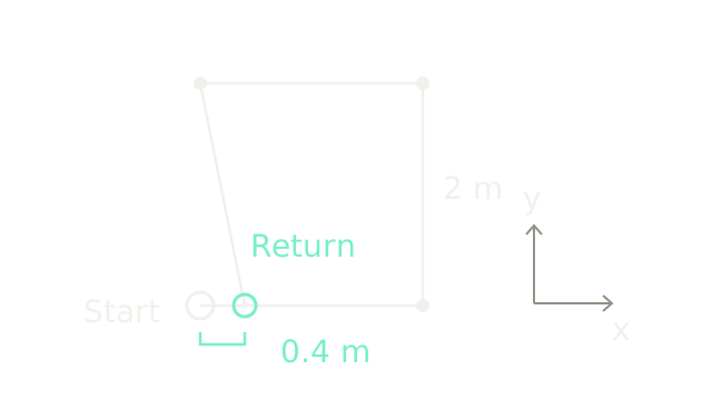
Now switch to a separate two-dimensional example at 100 pixels per metre on both axes. Assume known orientation and four measured translations: $(2,0)$, $(0,2)$, $(-2,0)$ and $(0.4,-2)$ m. Their sum is $(0.4,0)$, so the odometry path ends 40 pixels right of its start. The white starting ring and mint return ring remain separate.

A verified observation that this is the starting place supplies a loop-closure constraint. It connects the present estimate to an earlier pose; it is additional evidence, rather than an instruction to erase all error. The GTSAM PoseSLAM example adds such a factor between revisited poses without requiring explicit landmark variables. Here the proposed return has zero relative translation; the next beat declares exactly how strongly it is enforced.

Spread the correction

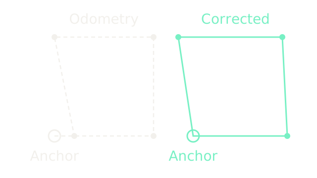
The two panels use identical 100-pixels-per-metre scales and keep their starting rings fixed. For a solvable limiting case, enforce the return exactly and give all four translation measurements the same independent isotropic variance. The least-squares solution subtracts $(0.1,0)$ m from each increment, removing the total 0.4-metre discrepancy with equal corrections. The corrected positions are

$$(0,0),\quad(1.9,0),\quad(1.8,2),\quad(-0.3,2),\quad(0,0)\text{ m}.$$

The upper corners move as well as the endpoint. Moving only the last pose would concentrate the correction in one edge and produce a larger squared-error sum under these equal weights. With a finite-noise return measurement, some closure residual generally remains; unequal covariances and orientation uncertainty change the distribution. The exact return drawn here is a declared simplification, not SLAM's usual promise.

Global corrections also need careful integration with control. ROS REP-105 distinguishes a continuous, drifting odom reference from a map reference that may jump when localization corrects. These are ROS conventions; a revised global estimate need not become an instantaneous physical motion command.

Where it breaks

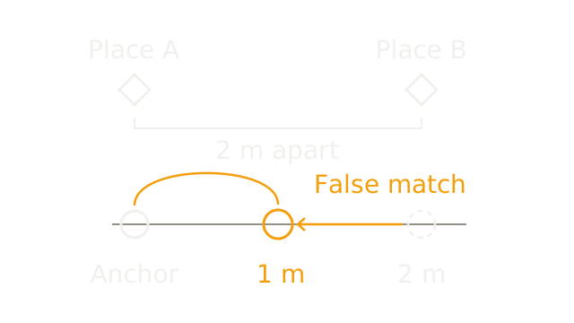
In this final independent example, two similar places A and B are really 2 m apart. Anchor A at zero. Odometry correctly reports a 2-metre displacement to B, but a false place match claims the robot returned to A, supplying a zero-displacement constraint. The lower ruler zooms to 160 pixels per metre: the dashed ring marks odometry's 2 m, while the amber ring shows the wrong compromise at 1 m.

If both constraints receive variance 0.04 m², the resulting objective is

$J(x)=\frac{(x-2)^2}{0.04}+\frac{x^2}{0.04},\qquad x^*=1\text{ m}.$

The optimizer has minimized the supplied cost correctly and still produced a physically wrong estimate. A believable-looking map cannot validate the correspondence that created it. Geometric verification and consistency tests belong before accepting a loop; robust residual models can reduce outlier influence. None guarantees rejection of a coherent false match in a repetitive environment.

The static-landmark assumption also matters: treating a moving object as a permanent reference inserts incompatible constraints. Calibration, timing, unobservable motion and poor initialization can fail even with correct identities. SLAM supplies an uncertain spatial estimate; motion planning still needs appropriate geometry and execution limits.

The Quick Version

• Relative observations leave the whole map's translation ambiguous.
• Anchoring a pose chooses coordinates, not global ground truth.
• Noisy motion increments accumulate into uncertain pose estimates.
• Reobserving landmarks exposes disagreement between predictions and measurements.
• Data association decides whether observations describe the same landmark.
• Factors connect noisy measurements to shared pose and map variables.
• Joint optimization can revise past poses and landmarks together.
• Loop closure relates a return observation to an earlier pose.
• Corrections spread according to constraints, geometry and uncertainty.
• False matches can make a correctly optimized estimate physically wrong.

Sources

Dellaert, Factor Graphs and GTSAM, especially the motion, PoseSLAM and landmark-SLAM examples, establishes the factor-graph construction. GTSAM's robust noise-model discussion covers outlier influence and robust estimation. ROS REP-105 defines the ROS map and odom distinction. All measured values, trajectories and numerical solutions on this page are synthetic teaching fixtures computed for these drawings.