Robot Localization and Mapping

Navigating an autonomous robot requires answering two coupled questions: where am I, and what does the surrounding world look like? Localization assumes a known map, mapping assumes known robot poses, and SLAM solves both concurrently while managing accumulating drift through loop closures.

Why Does This Exist?

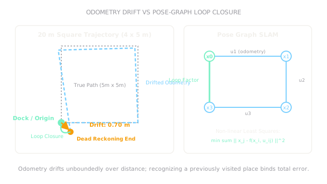
To navigate from an office desk to a charging dock, a mobile robot must know where it is in the world. If you rely solely on dead reckoning—integrating wheel encoder rotations and IMU gyroscopes step by step—your position estimate inevitably drifts. Wheel slip, uneven flooring, and tiny tire diameter differences accumulate without bound: after driving just twenty meters, the robot's internal odometer can be off by almost a meter.

If the robot plans its path using that drifting coordinate frame, it attempts to dock inside a solid plaster wall.

Robotic navigation resolves this by dividing the problem into three operational paradigms:

Localization: Given a pre-built reference map, determine the robot's current pose relative to that map.
Mapping: Given known, perfect robot poses, stitch sensory observations into an environment map.
SLAM (Simultaneous Localization and Mapping): When entering an unknown building with neither a map nor external GPS, estimate both the robot's trajectory and the environment geometry simultaneously.

Basics first: camera-based visual tracking and loop closure mechanics live in visual-slam. The sensor fusion filters that combine IMU and wheel encoders live in robot-state-estimation. Transforming coordinates between odometry, map, and base frames lives in robot-coordinate-frames.

Think of It Like This

Pacing through a strange misty maze with a blank notebook

Imagine you wake up in an unfamiliar hedge maze shrouded in thick mist. You have a blank notebook and a pencil. You start walking forward, counting paces: ten steps forward, turn ninety degrees right, ten steps forward. You sketch the corridors as you go.

Because your steps are not perfectly identical and your turns are not exactly ninety degrees, your hand-drawn sketch slowly skews and distorts.

After twenty minutes of walking, you round a corner and recognize a distinctive stone statue where you began. You realize: "I am back at the start!" That moment is a loop closure. You do not throw away your sketch: you use that single recognized landmark to pull the ends of your drawing together, retroactively untwisting the distorted corridors you paced out along the way.

Where it stops: humans recognize statues and textures through high-level semantic reasoning. A robotic SLAM stack matches LiDAR point scans or visual feature descriptors mathematically. If two distinct hallways look identical (perceptual aliasing), the robot can falsely close a loop, catastrophically warping a clean map into an unusable pretzel.

How It Actually Works

The navigation frame hierarchy: `map` versus `odom` versus `base_link`

Industrial robotics standards (like ROS REP-105) solve the drift problem by splitting navigation into three strictly separated coordinate frames:

base_link: Rigidly attached to the moving robot chassis.
odom (Odometry Frame): A continuous, smooth local coordinate frame. High-frequency wheel odometry and IMU integration update odom at $50\text{ Hz}$ to $200\text{ Hz}$ . It is guaranteed never to jump discontinuously, making it safe for low-level velocity and acceleration feedback control. However, it drifts unbounded over distance.
map (World Map Frame): A globally consistent, earth-fixed frame. Global localization (such as Monte Carlo Particle Filter or Graph-SLAM) periodically estimates the transform $\mathbf{T}_{\text{map} \leftarrow \text{odom}}$ . When a loop closure or landmark match occurs, this transform updates. It may jump discontinuously when corrections arrive.

The navigation stack routes global paths in map frame, but executes immediate obstacle avoidance and motor trajectory tracking in the smooth odom frame.

Pose-graph SLAM and loop closure

Modern SLAM formulates the problem as a factor graph:

Nodes $\mathbf{x}_i \in SE(2)$ or $SE(3)$ : The robot's historical poses at discrete timesteps.
Odometry Edges: Relative transformation constraints between consecutive poses: $\mathbf{z}_{i, i+1} = \mathbf{x}_i^{-1} \mathbf{x}_{i+1}$ .
Loop Closure Edges: Spatial constraints established when the robot recognizes a previously visited location: $\mathbf{z}_{i, j} = \mathbf{x}_i^{-1} \mathbf{x}_j$ where $j \ll i$ .

The full trajectory is solved via non-linear least squares optimization (using algorithms like Levenberg-Marquardt or Gauss-Newton):

\mathbf{X}^* = \arg\min_{\mathbf{X}} \sum_{(i,j) \in \mathcal{E}} \|\mathbf{z}_{ij} - \mathbf{h}(\mathbf{x}_i, \mathbf{x}_j)\|_{\boldsymbol{\Sigma}_{ij}}^2

When a loop closure constraint is added, the optimization distributes the accumulated residual drift evenly backward across the trajectory edges, pulling the entire map into global alignment.

Worked example: odometry drift across a 20-meter square loop

A mobile base drives a square path consisting of four straight legs of $5.0\text{ meters}$ each ( $20.0\text{ m}$ total perimeter).

Due to a slight wheel diameter mismatch or gyro calibration error, the robot incurs a systematic heading bias error of $+2.85^\circ$ ( $0.0497\text{ rad}$ ) on each $90^\circ$ turn.

Leg 1 (East, $0^\circ$ ): Starts at $(0.0, 0.0)$ , drives $5.0\text{ m}$ forward: $x_1 = 5.000\text{ m}, \quad y_1 = 0.000\text{ m}$
Turn 1: Commanded $90^\circ$ , actual heading $\theta_1 = 92.85^\circ$ .
Leg 2 (North): $x_2 = 5.000 + 5.0 \cos(92.85^\circ) = 5.000 - 0.248 = 4.752\text{ m}$ $y_2 = 0.000 + 5.0 \sin(92.85^\circ) = 0.000 + 4.994 = 4.994\text{ m}$
Turn 2: Commanded $90^\circ$ , actual heading $\theta_2 = 185.70^\circ$ .
Leg 3 (West): $x_3 = 4.752 + 5.0 \cos(185.70^\circ) = 4.752 - 4.975 = -0.223\text{ m}$ $y_3 = 4.994 + 5.0 \sin(185.70^\circ) = 4.994 - 0.496 = 4.498\text{ m}$
Turn 3: Commanded $90^\circ$ , actual heading $\theta_3 = 278.55^\circ$ .
Leg 4 (South): $x_4 = -0.223 + 5.0 \cos(278.55^\circ) = -0.223 + 0.743 = +0.520\text{ m}$ $y_4 = 4.498 + 5.0 \sin(278.55^\circ) = 4.498 - 4.944 = -0.446\text{ m}$

At the end of the four legs, open-loop dead reckoning expects to be back at $(0.0, 0.0)$ . Instead, the robot's actual estimated position has drifted to $(0.520, -0.446)\text{ m}$ .

The accumulated Cartesian drift magnitude is:

\Delta = \sqrt{0.520^2 + (-0.446)^2} = \sqrt{0.2704 + 0.1989} = \sqrt{0.4693} \approx 0.685 \approx 0.70\text{ m}

When the robot observes the starting docking station with its LiDAR scanner, a loop-closure edge binds the current pose $\mathbf{x}_4$ back to $\mathbf{x}_0$ , eliminating the $0.70\text{ m}$ discrepancy across the graph.

Code

This Python snippet simulates the 4-leg square loop with heading bias, computes the accumulated drift vector, and demonstrates how a loop-closure constraint closes the trajectory.

1import math2
3
4def simulate_square_odometry_drift(5    leg_length_m: float = 5.0,6    turn_bias_deg: float = 2.85,7) -> tuple[float, float, float]:8    """Simulate a 4-leg square loop with angular turn bias and return final drift."""9    x: float = 0.010    y: float = 0.011    theta_rad: float = 0.012
13    for _ in range(4):14        # Drive forward one leg15        x += leg_length_m * math.cos(theta_rad)16        y += leg_length_m * math.sin(theta_rad)17        # Turn 90 degrees plus systematic bias18        theta_rad += math.radians(90.0 + turn_bias_deg)19
20    drift_mag: float = math.hypot(x, y)21    return round(x, 3), round(y, 3), round(drift_mag, 2)22
23
24drift_x, drift_y, total_drift = simulate_square_odometry_drift()25print(drift_x)      # -> 0.5226print(drift_y)      # -> -0.44627print(total_drift)  # -> 0.69

Watch Out For

Planning local motor trajectories directly in the global map frame

Because global localization (such as adaptive Monte Carlo localization) periodically updates against landmarks, the transform $\mathbf{T}_{\text{map} \leftarrow \text{odom}}$ can jump by several centimeters or degrees when a new scan matches.

If low-level motor controllers evaluate tracking error directly in the map frame, that instantaneous discrete jump looks like an infinite velocity spike, causing the robot to violently jerk its steering motors. Fix it by separating frame responsibilities: compute global waypoints in map, but transform the active local trajectory into the continuous odom frame for low-level PID control.

Perceptual aliasing causing false loop closures

In symmetrical environments (such as long office corridors with identical doorways or warehouse racking aisles), a scan-matching algorithm can find a high-scoring match with an entirely different aisle that looks identical.

The symptom is a catastrophic corruption of the pose graph: the optimizer forces two distant corridors to occupy the same physical coordinates, twisting the map into an unnavigable mess. Fix it by requiring multi-hypothesis verification, geometric consistency checks over a window of consecutive poses, and rejecting candidate loop closures with high Mahalanobis distance.

The Quick Version

Mobile robot navigation separates localization (finding pose in a known map) from mapping (building a map from known poses) and SLAM (solving both together).
Open-loop dead reckoning accumulates drift without bound: over a $20\text{ m}$ square loop, a $2.85^\circ$ heading turn bias causes nearly $0.70\text{ m}$ of position drift.
Navigation architectures maintain three distinct frames: base_link (chassis), odom (smooth, continuous local tracking), and map (globally consistent, non-drifting world frame).
Loop closure is the critical mechanism of SLAM: recognizing a previously visited landmark introduces an optimization constraint that eliminates accumulated drift across the entire graph.
Perceptual aliasing in repetitive corridors must be guarded against to prevent false loop closures from corrupting the spatial map.