Binary Image Classification

Binary image classification answers one yes-or-no question per photo, such as defect or clean, with a single sigmoid output instead of a full multi-class head.

A binary image classifier maps a photo to one probability through a single sigmoid output, flagging it as positive or negative.

Why Does This Exist?

Most applied vision questions are yes-or-no: defect or clean, tumor or healthy, spam or not. Image classification covers the general machinery, but the two-class case deserves its own page because the head, the loss and the threshold decision all simplify, and the failure modes differ. There is no runner-up class to inspect, so calibration and the decision threshold carry the whole deployment.

Think of It Like This

A bouncer with one rule

A bouncer checking a single rule, over 21 or not, needs one glance at one ID field and one yes-or-no call. They do not rank the patron against every person in the city.

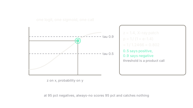
A binary head is that bouncer. One logit, one sigmoid, one threshold, typically 0.5. Everything else in the network just prepares the evidence for that single call.

How It Actually Works

Head, loss and threshold

The backbone produces a feature vector, and one linear unit outputs a logit $z$ . The predicted probability is $p = \sigma(z) = 1 / (1 + e^{-z})$ , where $\sigma$ is the sigmoid function mapping any real number into $(0, 1)$ . Training minimizes binary cross-entropy $L = -(y \log p + (1 - y) \log (1 - p))$ , where $y$ is 1 for positive and 0 for negative.

At inference you compare $p$ against a threshold $\tau$ , usually 0.5. Raise $\tau$ to 0.8 and you trade recall for precision: fewer false alarms, more missed positives. That tradeoff is a product decision, not a model property, and it is the main reason binary heads stay deployed for years.

A worked example

A chest X-ray head outputs $z = 1.4$ . Then $p = 1 / (1 + e^{-1.4}) \approx 1 / (1 + 0.2466) \approx 0.802$ . At $\tau = 0.5$ the scan is flagged positive with 80% confidence. Move $\tau$ to 0.9 and the same scan flips to negative, which is correct behavior if false alarms page a radiologist at 3am.

Code

1import torch2
3head = torch.nn.Linear(2048, 1)4criterion = torch.nn.BCEWithLogitsLoss()5
6features = torch.randn(8, 2048)          # backbone output for 8 images7labels = torch.tensor([1., 0., 1., 1., 0., 0., 1., 0.]).unsqueeze(1)8
9logits = head(features)10loss = criterion(logits, labels)11probs = torch.sigmoid(logits)12predicted = (probs > 0.5).long()

Watch Out For

Accuracy lies under class imbalance

With 95% negatives, a model that always answers negative scores 95% accuracy while catching nothing. The symptom is a great accuracy number beside a recall near zero. Report precision, recall and the confusion matrix, and consider weighting the positive class in the loss.

Shipping the default 0.5 threshold

The 0.5 default assumes false positives and false negatives cost the same, which is rarely true in medicine or manufacturing. Tune $\tau$ on validation data against real costs before deployment, and re-tune it when the class ratio shifts.

The Quick Version

Binary image classification answers one yes-or-no question per photo with a single sigmoid output.
Training uses binary cross-entropy on the logit; inference thresholds the probability.
The threshold trades precision against recall and is a product decision.
Under imbalance, accuracy misleads, so report precision, recall and the confusion matrix.