Convolutional Layers

Small shared filters scan the image and fire wherever their pattern appears, turning millions of pixels into stacked feature maps with few weights.

A 3x3 filter slides over a 5x5 image and writes one match score per position, so a Sobel patch scoring 4 marks a vertical edge in the 3x3 output

Why Does This Exist?

A $1000 \times 1000$ color image holds three million values. Feeding that into a single hidden layer of just 1000 dense neurons needs three billion weights — one per pixel per neuron — and it treats a cat in the top-left corner as unrelated to the same cat in the bottom-right. Brute force fails on memory, on compute, and on the spatial structure of images.

Convolutional layers solve all three with two properties of the visual world: patterns are local, and a pattern means the same thing wherever it appears. Each neuron watches only a small patch, and every position shares the same filter weights. Early layers learn edges, deeper layers combine them into shapes, and translation comes free. This page covers the layer itself. How size is preserved or halved is in padding and stride, what the outputs look like in feature maps, and how resolution is pooled in pooling and downsampling.

The one idea you need first

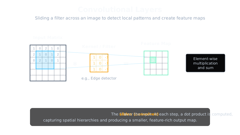
A dot product multiplies two equal-length lists element-wise and sums the results into one number. A convolution is that operation repeated: at each position, dot the filter weights with the image patch beneath, and write the single score into the output. High score means the pattern is there.

Think of It Like This

Searching a dark room with a flashlight

Imagine a dark room where you hunt lost keys with a flashlight that lights only a small circle — the receptive field. You sweep it left to right, top to bottom, checking each lit patch for the key shape with the same eyes at every stop.

The image is the room, the filter is the beam, and the sweep is the stride. The analogy stops at the sharing: you could choose to look for something different in each corner, but the layer is forbidden to — identical weights everywhere is exactly what buys translation invariance and the tiny parameter count.

How It Actually Works

A filter is a small matrix of weights, typically $3 \times 3$ or $5 \times 5$ , whose values decide which pattern it detects — learned by backpropagation, not hand-set. It slides over the image in steps of the stride $S$ , and at each stop the dot product of weights with the patch becomes one output number. Those scores tile into a feature map. A real layer stacks dozens of filters: with a 3-channel input each filter has depth 3 and dots across all channels at once, so 64 filters on RGB produce 64 output channels.

Output size follows one formula. For input width $W$ , filter $F$ , padding $P$ and stride $S$ , the output width is $(W - F + 2P) / S + 1$ . A $5 \times 5$ image with a $3 \times 3$ filter, stride 1 and no padding gives $(5 - 3) / 1 + 1 = 3$ : a $3 \times 3$ feature map.

Worked example

Take a $5 \times 5$ image holding a $3 \times 3$ block of ones (a white square on black) and a vertical-edge Sobel filter with left column $[-1, -2, -1]$ , middle zeros, right column $[1, 2, 1]$ . At the middle-left output position the patch straddles the square's left border — zeros left, ones middle and right — so the score is $0 + 0 + (1 + 2 + 1) = 4$ . The full $3 \times 3$ output is $[[3, 0, -3], [4, 0, -4], [3, 0, -3]]$ : positive down the left (dark-to-light edge), negative down the right (light-to-dark), zeros in the uniform middle. One filter, one sweep, both borders found.

Code

The worked example in PyTorch, applying a Sobel filter to the white square:

1import torch2import torch.nn.functional as F3
4# 1. Dummy 5x5 image (1 batch, 1 channel) with a 3x3 block of ones5image = torch.tensor([6    [0.0, 0.0, 0.0, 0.0, 0.0],7    [0.0, 1.0, 1.0, 1.0, 0.0],8    [0.0, 1.0, 1.0, 1.0, 0.0],9    [0.0, 1.0, 1.0, 1.0, 0.0],10    [0.0, 0.0, 0.0, 0.0, 0.0]11]).view(1, 1, 5, 5)12
13# 2. 3x3 vertical-edge Sobel filter14kernel = torch.tensor([15    [-1.0, 0.0, 1.0],16    [-2.0, 0.0, 2.0],17    [-1.0, 0.0, 1.0]18]).view(1, 1, 3, 3)19
20# 3. Convolve: (5 - 3) / 1 + 1 = 3, so output is 1x1x3x321feature_map = F.conv2d(image, kernel, stride=1, padding=0)22
23print(feature_map)24# -> tensor([[[[ 3.,  0., -3.],25# ->           [ 4.,  0., -4.],26# ->           [ 3.,  0., -3.]]]])

The printed map matches the hand computation exactly: $+4$ on the rising edge, $-4$ on the falling edge.

Watch Out For

Forgetting spatial dimensions with no padding

A $3 \times 3$ filter on a $32 \times 32$ image without padding gives $30 \times 30$ . Stack ten such layers and the map shrinks to $12 \times 12$ before any pooling — deep stacks can vanish entirely. The symptom is shape-mismatch errors in skip connections or a map too small to detect anything.

Choose padding deliberately (padding=1 preserves size for $3 \times 3$ stride-1) whenever the architecture assumes resolution survives the layer.

Misunderstanding filter depth vs output channels

A single filter must always be as deep as its input (3 for RGB), and the number of filters sets the output channels: 64 filters make 64 channels regardless of input depth. The symptom is a weight tensor built with the wrong shape, or surprise at a layer's parameter count.

Read weight shapes as (out-channels, in-channels, height, width) and the confusion disappears.

The Quick Version

Convolutional layers reuse small shared filters across the image, cutting three billion dense weights to thousands.
Each output is a dot product of filter weights with the patch beneath: high score means the pattern is there.
Output width follows $(W - F + 2P) / S + 1$ ; a 5x5 image with a 3x3 stride-1 filter gives 3x3.
A Sobel sweep finds both borders of a white square in one pass: +4 rising, -4 falling.
One layer stacks dozens of filters, each as deep as the input, producing a volume of feature maps.
Stride and padding govern output size, so set them deliberately in deep stacks.