Inductive Bias Theory

Data never picks a unique model, so every learner smuggles preferences. Inductive bias names those preferences: the locality, smoothness, and simplicity a network favors before seeing data.

Two-point averaging erases the alternating signal completely while preserving the smooth ramp, the low-frequency preference in one picture

Why Does This Exist?

No dataset determines a unique model: infinitely many functions fit any finite training set, from smooth laws to lookup tables with spikes. Yet gradient-trained networks keep landing on the smooth ones that generalize. The data cannot explain that — the learner's preferences do, and unnamed preferences cannot be audited.

Inductive bias theory names them: convolutional locality, spectral bias toward low frequencies, simplicity bias toward easy features, and the texture preference that follows. It explains generalization where parameter counts cannot, and predicts failure where the bias mismatches the world. The gap view is generalization theory; the scaling view is scaling laws.

The one idea you need first. No free lunch says no learner wins everywhere: every edge on some tasks is paid for on others. An architecture's bias is its prepaid choice of which tasks to win — CNNs prepay for local, translation-stable patterns and underpay for long-range arithmetic. Reading a model means reading what it prepaid.

Think of It Like This

A judge's sentencing guidelines

Two judges apply the same law and reach different sentences: the law sets the range, but each judge's guidelines supply defaults — first offenders get leniency, remorse counts double. The guidelines decide every case the law leaves open, which is most cases.

Training data is the law: it rules out wrong models but leaves a vast legal range. Architecture and optimization are the guidelines: locality, smoothness, and simplicity defaults that pick the sentence. Appeals (distribution shift) reveal the guidelines exactly where they diverge from justice — texture bias sails training and fails sketches, because the default was texture all along.

How It Actually Works

Biases compose across scales. Architectural: convolutions see locally and share across positions; attention sees globally but permutes freely. Spectral: networks fit low frequencies first, so smooth structure precedes fine detail during training. Simplicity: among zero-error fits, gradient descent drifts toward low-norm, compressible solutions. Texture: standard training on natural photos rewards local statistics over global shape, so cue-conflict images (cat shape, elephant skin) get labeled by skin.

Each bias is a bet. Locality wins on photos, loses on counting and arithmetic. Spectral bias wins on natural scenes, loses on high-frequency codes. Auditing means listing the bets and testing each against shifted data.

Worked example

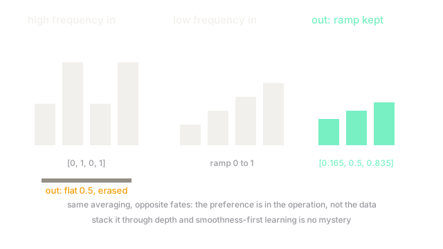
A two-point moving average is the simplest low-pass preference. Alternating signal $[0, 1, 0, 1]$ (pure high frequency) averages to $[0.5, 0.5, 0.5]$ : amplitude $0.5$ in, $0$ out — erased completely. Smooth ramp $[0, 0.33, 0.67, 1.0]$ averages to $[0.165, 0.5, 0.835]$ : the shape survives with mild shrinkage.

Same operation, opposite fates: high frequencies die, low frequencies pass. Stack such preferences through depth and training order, and the network's famous smoothness-first learning is no mystery — it is averaging all the way down.

Code

The point of this snippet is the preference made mechanical: one averaging pass kills oscillation and keeps the ramp.

1def moving_average(signal: list) -> list:2    return [(signal[i] + signal[i + 1]) / 2.0 for i in range(len(signal) - 1)]3
4
5print(moving_average([0.0, 1.0, 0.0, 1.0]))  # -> [0.5, 0.5, 0.5]6print(moving_average([0.0, 0.33, 0.67, 1.0]))  # -> [0.165, 0.5, 0.835]

Watch Out For

Helpful bias becomes shortcut under shift

Texture bias is free accuracy on photo test sets and a trap on sketches, silhouettes, and stylized inputs, where shape-believing humans sail and texture-believing models sink. The bias never announces itself; only shifted evaluation exposes it.

Evaluate on cue-conflict and style-shifted slices before deployment claims. When bias and task diverge, intervene at the source: shape-biased augmentation, texture dropout, or architectures with global structure.

Mistaking the default for understanding

A model that answers smoothly and simply looks like it reasons — until a task needs the dispreferred skill (counting, parity, long-range dependency) and it fails with the same confidence. Simplicity bias manufactures fluent wrongness.

Probe dispreferred skills deliberately: counting, relational chains, high-frequency codes. Fluency is the bias talking; the probes check whether anything else is home.

The Quick Version

Inductive bias is the learner's prepaid preference ordering over the models data leaves open.
The worked fixture erases $[0, 1, 0, 1]$ to flat $0.5$ while preserving a ramp: low frequencies pass.
Locality, spectral bias, and simplicity compose into smoothness-first learning.
Texture preference is free accuracy on photos and a trap on sketches and silhouettes.
Audit each bet with shifted evaluation; fluency alone never proves understanding.