Mixup Augmentation
Blend two photos and blend their labels with the same weight. The model learns smooth transitions instead of memorizing sharp borders.
Why Does This Exist?
One hot labels claim every photo is fully one thing. Real decision borders are softer, and models trained on hard corners grow overconfident between them. A 0.51 dog still reports 0.99 dog, which breaks ranking and thresholding downstream.
Mixup builds the soft middle directly. Take two labeled photos, blend every pixel with weight , and train on the blended label with the same . The network must output 0.7 dog for a 0.7 blend, which smooths the border. It complements cutout, which erases instead of blending, and the family overview is image augmentation.
You need one idea first. A label can be a distribution, not a single spike. Mixup manufactures those distributions from pairs you already have.
Think of It Like This
Two paint cans poured together
Pour 70 percent white and 30 percent gray into one bucket and the result is light gray, honestly labeled 0.7 and 0.3. Nobody calls it pure white.
Mixup pours pixels the same way. The blended photo is 0.7 first class and 0.3 second, and the loss grades that exact claim. Where the analogy stops: paint mixes physically, while pixels blend numerically with no new scene behind them.
How It Actually Works
The blend rule
Draw from with often to . Given images and one hot labels :
Training minimizes cross entropy against , which equals times the loss on plus times the loss on . No box moves, because every pixel is a mix.
A worked pixel and label
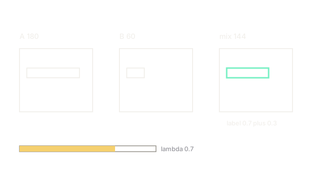
, pixel , pixel :
Label and become . The model must report 70 percent first class on this ghost, which is the smoothing supervision hard labels never give.
Setting alpha
Small near keeps near 0 or 1, so blends stay readable. samples uniformly and makes stronger ghosts. Start at for small datasets and raise only if calibration stays poor.
Code
import numpy as np
def mixup_pair(a: np.ndarray, b: np.ndarray, lam: float) -> np.ndarray: """Convex blend of two float images with weight lam.""" return lam * a + (1.0 - lam) * b # same lam blends the labels
a = np.array([180.0])b = np.array([60.0])print(mixup_pair(a, b, 0.7).tolist()) # -> [144.0]Watch Out For
Ghosts near one half confuse small objects
At near neither class dominates, and a tiny bird blended half with sky becomes unlearnable noise with a confident 0.5 tag. The symptom is stalled tail accuracy while head classes smooth nicely. Keep small or skip mixup on tiny object slices.
Applying mixup to boxes without a plan
Blended pixels carry two scenes, but one box file cannot hold both truths. Naively keeping box teaches box as background. Use mixup for classification first, and reach for CutMix with area labels when boxes matter.
The Quick Version
- Mixup blends two images with weight lambda and blends their labels with the same lambda.
- A 0.7 blend of 180 and 60 gives pixel 144 with label 0.7 and 0.3.
- Lambda comes from a Beta distribution, often with alpha 0.2 for gentle blends.
- Keep alpha small on tiny objects and avoid mixup where boxes need exact labels.