Otsu Thresholding

Otsu thresholding picks the cutoff that minimizes within-class variance across the histogram, the best automatic split for bimodal images.

Otsu scans every candidate cutoff and keeps the one where the two resulting classes are tightest inside and farthest apart.

Why Does This Exist?

Global thresholding needs a human to find the histogram valley, which breaks automation: the next batch has different lighting and the valley moves. Otsu's method (Nobuyuki Otsu, 1979) finds the optimal cutoff from the histogram alone by trying every candidate and keeping the one that makes the two classes tightest. It is the zero-tuning default for bimodal images in inspection, microscopy and document pipelines, and the automatic member of the thresholding trio. Pass cv2.THRESH_OTSU as a flag and OpenCV returns the chosen cutoff alongside the mask.

This page covers the variance criterion, a fully hand-scored six-level example, and the bimodality assumption that bounds it.

Think of It Like This

Splitting a tug-of-war roster by weight

A coach must split players into light and heavy teams with one weight cutoff, and wants both teams internally even. Trying every candidate split and measuring the spread inside each team, the coach picks the split with the smallest combined spread. That is Otsu: every histogram level is a candidate cutoff, tightness is variance, and the best split minimizes it.

The analogy stops at two teams. The coach never asks whether three teams fit better. Otsu likewise assumes exactly two classes; a three-hump histogram gets force-split into two, and the answer is confidently wrong.

How It Actually Works

The variance criterion

For candidate cutoff $T$ , split pixels into class 0 (levels $\le T$ ) and class 1 (levels $> T$ ) with weights $w_0, w_1$ and means $\mu_0, \mu_1$ . The between-class variance is $\sigma_b^2(T) = w_0 w_1 (\mu_0 - \mu_1)^2$ . Maximizing it equals minimizing within-class spread, but needs only class weights and means, so all 256 candidates score in microseconds. The $T$ with the largest $\sigma_b^2$ wins; ties resolve to the first maximum in most implementations.

Worked six-level example

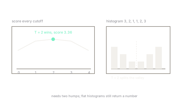
Histogram counts $[3, 2, 1, 1, 2, 3]$ over levels 0 to 5 (12 pixels, humps at both ends). Scoring each candidate:

$T = 0$ : classes $\{0\}$ vs rest, $\sigma_b^2 = 2.0833$
$T = 1$ : $\{0, 1\}$ vs rest with $\mu_0 = 0.4$ , $\mu_1 = 4.0$ , $\sigma_b^2 = 3.1500$
$T = 2$ : $\mu_0 = 0.667$ , $\mu_1 = 4.333$ , $\sigma_b^2 = 3.3611$
$T = 3$ : symmetric to $T = 1$ , $\sigma_b^2 = 3.1500$
$T = 4$ : symmetric to $T = 0$ , $\sigma_b^2 = 2.0833$

The unique peak at $T = 2$ sits exactly in the valley between the humps, which is the result you would pick by eye, now derived. Pixels above 2 become foreground.

The bimodality contract

Otsu assumes two classes and roughly comparable spreads. Unimodal histograms (a single hump) still return a "best" split that segments noise; heavily imbalanced classes drag the cutoff into the majority hump; gradients across the frame smear the humps together. Validate with the histogram plot and a glance at the mask. For three or more real classes, use multi-Otsu (threshold_multiotsu in scikit-image); for uneven light, use adaptive.

Code

1counts = [3, 2, 1, 1, 2, 3]  # 12 pixels over levels 0..52N = sum(counts)3
4def sigma_b(T):5    w0 = sum(counts[:T + 1]) / N6    w1 = 1 - w07    m0 = sum(i * c for i, c in enumerate(counts[:T + 1])) / sum(counts[:T + 1])8    m1 = sum(i * c for i, c in enumerate(counts[T + 1:], start=T + 1)) / sum(counts[T + 1:])9    return w0 * w1 * (m0 - m1) ** 210
11scores = [(T, round(sigma_b(T), 4)) for T in range(5)]12print(scores)13# -> [(0, 2.0833), (1, 3.15), (2, 3.3611), (3, 3.15), (4, 2.0833)]

Watch Out For

Confident splits of unimodal histograms

Otsu always returns a threshold, even when no two classes exist. The symptom is a "segmentation" of pure noise or a clean background into arbitrary halves. Never trust the number alone: plot the histogram for two humps and eyeball the mask before automating.

Forgetting the flag returns zero

Calling cv2.threshold with $T = 0$ but without THRESH_OTSU just cuts at zero instead of searching. The symptom is an all-white mask and a returned threshold of 0. The call must read cv2.threshold(gray, 0, 255, cv2.THRESH_BINARY + cv2.THRESH_OTSU) so the flag triggers the search.

The Quick Version

Otsu tries every cutoff and maximizes $\sigma_b^2 = w_0 w_1 (\mu_0 - \mu_1)^2$ .
Example: counts $[3,2,1,1,2,3]$ peak uniquely at $T = 2$ with 3.3611.
Zero-tuning and automatic, via the THRESH_OTSU flag with $T = 0$ passed in.
Assumes exactly two classes; force-splits unimodal and trimodal histograms wrongly.
Imbalanced classes and lighting gradients need adaptive or multi-Otsu instead.