scikit-image Filters for Vision

A NumPy-first toolbox of image filters, segmentation and measurements, so small array experiments teach the operation before any model runs.

scikit-image turns a small step patch into a measured gradient of 10

Why Does This Exist?

OpenCV moves pixels fast, but its functions hide the math behind flags and defaults. When you are learning, or debugging a pipeline, you want each operation spelled out on a small array: this filter, this patch, this number. scikit-image is built for that. Every function takes a NumPy array and returns one, with names that match textbooks, so basic operations stay inspectable.

This page covers purpose, the array I/O contract, one gradient fixture, and appropriate use. Color meanings live in color spaces. The 0.26 series was the current stable line verified in-session.

Think of It Like This

A measuring bench beside the power tools

A workshop has power saws that cut fast and a measuring bench with rulers and calipers. You shape stock at the bench first, where every cut is visible and reversible, and only then run the production saw.

scikit-image is the bench. Arrays go in, measured arrays come out, and each step prints its numbers. The analogy stops at speed: the bench is slower on huge images, which is why production pipelines still reach for compiled loaders after the math is settled.

How It Actually Works

Input is a NumPy array, either grayscale $(H, W)$ or color $(H, W, C)$ , usually float in $[0, 1]$ for filters. Output is another array of the same family: a filtered image, a labeled mask, or a table of region properties. Purpose is research-grade reference operations: gradients, thresholding, morphology, segmentation, and measurement, each with one clear call. Appropriate use is experiments, teaching, and pipeline checks on small crops. For video-rate loading, pair it with a faster reader and keep scikit-image for the analysis step.

Step patch fixture

Take a 3 by 3 patch that steps from 0 to 10 down the middle:

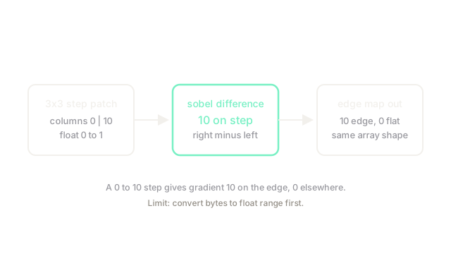
\begin{bmatrix} 0 & 10 & 10 \\ 0 & 10 & 10 \\ 0 & 10 & 10 \end{bmatrix}

A horizontal difference filter reads right minus left at the edge column, giving $10 - 0 = 10$ . Flat columns give 0. So the response is 10 exactly on the step and 0 elsewhere, which is the diagram's claim: edges are places where the difference is large, and the number says how large.

Code

The same difference in plain Python, mirroring the filter call:

1def edge_response(left: float, right: float) -> float:2    return right - left  # one horizontal difference at the step3
4
5print(edge_response(0.0, 10.0))  # -> 10.06print(edge_response(10.0, 10.0))  # -> 0.0

Step columns give 10.0, flat columns give 0.0, which is what the filter array reports at each pixel.

Watch Out For

Filtering 0 to 255 bytes as if they were 0 to 1 floats

Many scikit-image filters assume float input in $[0, 1]$ . The symptom is a threshold or gradient that behaves wildly on a uint8 array: values 200 times larger than the defaults expect. Fix it by converting once on entry and keeping the range beside the shape in every check.

The Quick Version

scikit-image maps NumPy arrays to filtered arrays, masks, or region tables with textbook names.
Inputs are grayscale or color arrays, best as float in 0 to 1 for filter calls.
A 0 to 10 step gives a gradient response of 10 on the edge and 0 on flat ground.
Use it for experiments and checks, with faster readers handling bulk loading.
Convert byte images to float range once, or thresholds misbehave silently.