Alternative Novel Architectures

Alternative architectures break free from static discrete layer stacks by modeling continuous depth, adaptive time constants, and linear recurrence.

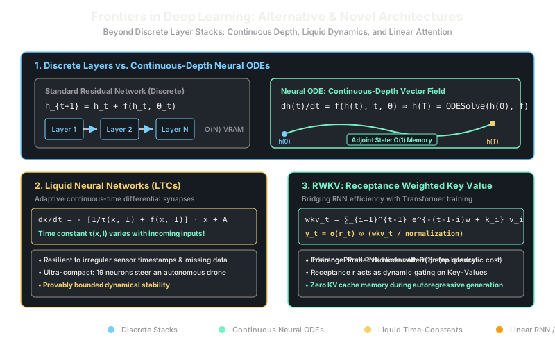
Comparing paradigm shifts: continuous-depth Neural ODEs, input-adaptive Liquid Neural Networks, and linear-attention RWKV architectures

Why Does This Exist?

The contemporary deep learning landscape is dominated by two architectural archetypes: Multi-Layer Perceptrons (feed-forward-networks) and Attention-based transformers. While undeniably effective at scale, these architectures carry entrenched systemic compromises:

Discrete Layer Stacks Require Fixed Compute: A 64-layer Transformer executes exactly 64 sequential matrix operations whether answering "What is 2+2?" or synthesizing quantum physics. It cannot adapt its computational depth to the difficulty of the input.
Backpropagation Through Depth Demands $O(D)$ Activation Memory: Standard backpropagation requires caching intermediate activations at every single layer $1, 2, \dots, D$ , consuming tens of gigabytes of GPU VRAM strictly for gradient computation.
Quadratic Sequence Scaling and KV Cache Inefficiency: Standard softmax self-attention scales as $O(L^2)$ in time and $O(L)$ in state memory, making edge robotics and million-token reasoning prohibitively expensive.
Failure on Irregularly Sampled Time Series: Standard recurrent and convolutional networks assume inputs arrive at perfectly uniform clock intervals ( $\Delta t = \text{const}$ ). In real-world edge sensing, medical telemetry, and robotics, signals arrive with arbitrary, noisy time gaps.

Alternative and Novel Architectures break outside the discrete-layer Transformer orthodoxy. By reformulating neural computation through continuous dynamical systems, bio-inspired liquid time constants, and linear-time recurrent formulations, these models pioneer radically higher parameter efficiency, continuous-depth reasoning, and constant-memory inference.

Think of It Like This

A digital clock stepper vs a hydraulic fluid flow

Standard neural networks like ResNets and Transformers operate like a digital quartz clock. Every tick of the clock is a discrete layer: tick 1 executes Layer 1, tick 2 executes Layer 2. If a sensor reading arrives between ticks, the clock cannot register it without interpolating or padding. If you want more precision, you must physically solder more discrete clock gears into the chassis ( $O(D)$ memory).

Neural Ordinary Differential Equations (Neural ODEs) replace the clock gears with a continuous hydraulic fluid pipeline. The inputs are injected as a dye droplet into a flowing fluid whose velocity vector field is parameterized by a neural network. To compute the answer, you do not count discrete layers; you simply open the valve and integrate the fluid flow over time using a numerical solver. If you need a fast answer on a low-power microcontroller, you run a coarse solver with 3 big steps. If you need extreme scientific precision, you tighten the error tolerance and take 100 micro-steps—using the exact same network weights.

Liquid Neural Networks make the viscosity of the fluid itself dynamic: when sensor inputs change violently, the fluid liquefies and updates instantly; when inputs are quiet, it thickens, preserving memory without drifting.

How It Actually Works

Continuous Depth, Dynamic Time Constants, and Linear Recurrence

Three principal families define the modern frontier of alternative architectures:

1. Neural Ordinary Differential Equations (Neural ODEs)

A residual network computes discrete updates: $h_{t+1} = h_t + f(h_t, \theta_t)$ . In the limit of infinitesimal step size $\Delta t \to 0$ , this difference equation becomes a continuous ordinary differential equation:

\frac{dh(t)}{dt} = f(h(t), t, \theta)

The output state $h(T)$ is obtained by integrating from $t=0$ to $t=T$ using adaptive numerical ODE solvers (such as Runge-Kutta 4th/5th order or Dormand-Prince):

h(T) = h(0) + \int_0^T f(h(t), t, \theta) \, dt = \text{ODESolve}(h(0), f, 0, T)

Crucially, backpropagation does not require storing intermediate activations along the integration path. Using the Adjoint Sensitivity Method, gradients are computed by solving an auxiliary differential equation backwards in time:

\frac{da(t)}{dt} = -a(t)^T \frac{\partial f(h(t), t, \theta)}{\partial h}

where $a(t) = \frac{\partial \mathcal{L}}{\partial h(t)}$ is the adjoint state. This achieves constant $O(1)$ memory usage with respect to model depth.

2. Liquid Neural Networks (LNNs & LTCs)

Liquid Time-Constant (LTC) networks model continuous-time recurrent dynamics inspired by the nervous system of C. elegans. Unlike standard RNNs where synaptic weights are static, an LTC defines hidden states via non-linear differential equations where the effective time constant varies with inputs:

\frac{dx_i(t)}{dt} = -\left[ \frac{1}{\tau_i} + \sum_{j} w_{ij} \sigma(x_j(t)) \right] x_i(t) + \sum_{j} w_{ij} \sigma(x_j(t)) A_{ij} + I_i(t)

The system's adaptive time constant $\tau_{\text{eff}}(x, I) = \frac{\tau_i}{1 + \tau_i \sum w_{ij} \sigma(x_j)}$ automatically speeds up when high-frequency sensor perturbations occur and slows down during quiescent periods. This allows an ultra-compact 19-neuron liquid network to steer an autonomous drone directly from raw pixel feeds—a task typically demanding tens of millions of parameters in a CNN.

3. RWKV: Receptance Weighted Key Value

RWKV bridges the gap between Transformers and RNNs. It reinterprets attention as a linear recurrence with time-decay weighting:

R_t = \sigma(W_r x_t), \quad K_t = W_k x_t, \quad V_t = W_v x_t

The output is computed using an exponential decay accumulator:

\text{wkv}_t = \frac{\sum_{i=1}^{t-1} e^{-(t-1-i)w + K_i} V_i + e^{u + K_t} V_t}{\sum_{i=1}^{t-1} e^{-(t-1-i)w + K_i} + e^{u + K_t}}

Y_t = R_t \odot \text{wkv}_t

During training, this formulation is parallelized across sequence length $L$ in $O(L)$ time via prefix scans. During deployment, it executes as a pure RNN with $O(1)$ constant memory and zero KV cache growth.

Worked Example

Let us compare one forward step of a discrete Residual layer versus an explicit Euler numerical integration step of a Neural ODE:

Initial state $h_0 = [2.0, -1.0]^T$ . Let the neural vector field $f(h, \theta)$ be defined as:

f(h) = \begin{bmatrix} -0.5 \cdot h_1 \\ 0.2 \cdot h_0 \end{bmatrix}

1. Discrete Residual Block:

f(h_0) = \begin{bmatrix} -0.5(-1.0) \\ 0.2(2.0) \end{bmatrix} = \begin{bmatrix} 0.5 \\ 0.4 \end{bmatrix}

h_1 = h_0 + f(h_0) = \begin{bmatrix} 2.0 \\ -1.0 \end{bmatrix} + \begin{bmatrix} 0.5 \\ 0.4 \end{bmatrix} = \begin{bmatrix} 2.5 \\ -0.6 \end{bmatrix}

This is a rigid, fixed step.

2. Continuous Neural ODE with Adaptive Step Size $\Delta t$ :

Suppose the ODE solver determines that the gradient is steep and subdivides the interval $[0, 1]$ into two fine steps of $\Delta t = 0.5$ :

Step A ( $t = 0.0 \to 0.5$ ):

\frac{dh}{dt} = f(h_0) = \begin{bmatrix} 0.5 \\ 0.4 \end{bmatrix}

h(0.5) = h(0) + \Delta t \cdot f(h_0) = \begin{bmatrix} 2.0 \\ -1.0 \end{bmatrix} + 0.5 \begin{bmatrix} 0.5 \\ 0.4 \end{bmatrix} = \begin{bmatrix} 2.0 + 0.25 \\ -1.0 + 0.20 \end{bmatrix} = \begin{bmatrix} 2.25 \\ -0.80 \end{bmatrix}

Step B ( $t = 0.5 \to 1.0$ ): Re-evaluate the vector field at intermediate state $h(0.5)$ :

f(h(0.5)) = \begin{bmatrix} -0.5(-0.80) \\ 0.2(2.25) \end{bmatrix} = \begin{bmatrix} 0.40 \\ 0.45 \end{bmatrix}

h(1.0) = h(0.5) + \Delta t \cdot f(h(0.5)) = \begin{bmatrix} 2.25 \\ -0.80 \end{bmatrix} + 0.5 \begin{bmatrix} 0.40 \\ 0.45 \end{bmatrix} = \begin{bmatrix} 2.25 + 0.20 \\ -0.80 + 0.225 \end{bmatrix} = \begin{bmatrix} 2.45 \\ -0.575 \end{bmatrix}

By evaluating the intermediate velocity at $t=0.5$ , the continuous model curved accurately along the vector field, achieving higher numerical stability without adding extra parameters to the network.

Code

Below is a self-contained Python implementation of an explicit Euler solver simulating a continuous-depth Neural ODE forward trajectory:

1import numpy as np2
3
4class NeuralVectorField:5    """Parametric velocity field dh/dt = tanh(W h + b)."""6
7    def __init__(self, w: np.ndarray, b: np.ndarray):8        self.w = w9        self.b = b10
11    def __call__(self, h: np.ndarray) -> np.ndarray:12        return np.tanh(self.w @ h + self.b)13
14
15def ode_solve_euler(16    f: NeuralVectorField, h0: np.ndarray, t_start: float, t_end: float, steps: int17) -> tuple[np.ndarray, np.ndarray]:18    """Integrate dh/dt = f(h) from t_start to t_end using explicit Euler."""19    dt = (t_end - t_start) / steps20    trajectory = [h0.copy()]21    h = h0.copy()22
23    for _ in range(steps):24        dh_dt = f(h)25        h += dt * dh_dt26        trajectory.append(h.copy())27
28    return h, np.array(trajectory)29
30
31# Define a 2D neural vector field32w = np.array([[0.0, -1.2], [1.2, 0.0]])  # Rotational dynamics33b = np.array([0.1, -0.1])34field = NeuralVectorField(w, b)35
36h_initial = np.array([1.0, 0.0])37
38# Solve with coarse steps (fast inference)39h_coarse, _ = ode_solve_euler(field, h_initial, 0.0, 1.0, steps=2)40
41# Solve with fine steps (high precision)42h_fine, traj_fine = ode_solve_euler(field, h_initial, 0.0, 1.0, steps=10)43
44print(f"Initial state:   {h_initial}")45print(f"Coarse h(1.0):   {np.round(h_coarse, 4)}")46print(f"Fine h(1.0):     {np.round(h_fine, 4)}")47print(f"Trajectory shape: {traj_fine.shape}")48# -> Initial state:   [1. 0.]49# -> Coarse h(1.0):   [0.4566 0.9634]50# -> Fine h(1.0):     [0.4873 0.8872]51# -> Trajectory shape: (11, 2)

Watch Out For

Numerical solver stiffness causing runtime explosion in Neural ODEs

When training Neural ODEs, the optimizer can inadvertently learn highly oscillatory, chaotic vector fields $f(h, t, \theta)$ . When this happens, an adaptive-step ODE solver (like Dormand-Prince) is forced to take increasingly microscopic step sizes $\Delta t \to 0$ to satisfy local error tolerances. This phenomenon—known as stiffness—causes the Number of Function Evaluations (NFE) to explode from 20 steps to over 2,000 steps per forward pass, grinding training throughput to a halt. Always apply kinetic energy regularization or higher-order derivative penalties ( $\|\nabla_h f\|_F^2$ ) to keep the learned vector field smooth.

The Quick Version

Neural ODEs replace discrete layer stacks with continuous vector fields, using numerical solvers to integrate hidden states.
The Adjoint Sensitivity Method computes exact gradients backwards in time, yielding $O(1)$ constant memory scaling with model depth.
Liquid Neural Networks introduce input-dependent time constants that dynamically adapt to irregular, asynchronous sensor streams.
RWKV reinterprets attention as an exponential decay recurrence, enabling parallel training with constant-memory $O(1)$ inference.
Alternative architectures excel in scientific simulation, robotics, and edge deployment where Transformer memory footprints are unviable.