Kolmogorov-Arnold Networks

Why Does This Exist?

For nearly four decades, the Multi-Layer Perceptron (multi-layer-perceptron) has served as the foundational bedrock of deep learning, mathematically justified by the universal-approximation theorem. In an MLP, every incoming signal is multiplied by a static linear weight matrix $W$ along an edge, summed at the node (neuron), and passed through a fixed, non-linear activation function $\sigma$ (such as ReLU, GELU, or SiLU).

Despite their dominance, MLPs suffer from two fundamental weaknesses in scientific modeling and interpretability:

1. The Curse of Dimensionality in Approximation: To approximate high-frequency, complex multi-dimensional functions $f(x_1, \dots, x_d)$, standard MLPs require exponentially growing parameter counts ($O(\epsilon^{-d})$). They struggle to capture intricate local non-linearities without ballooning in size.
2. Total Black-Box Opacity: The weights in an MLP are uninterpretable matrix entries. Once trained, an MLP cannot tell an astrophysicist, fluid dynamicist, or pharmacologist what algebraic relationship it learned. It is nearly impossible to extract closed-form symbolic laws from an MLP's entangled weight space.

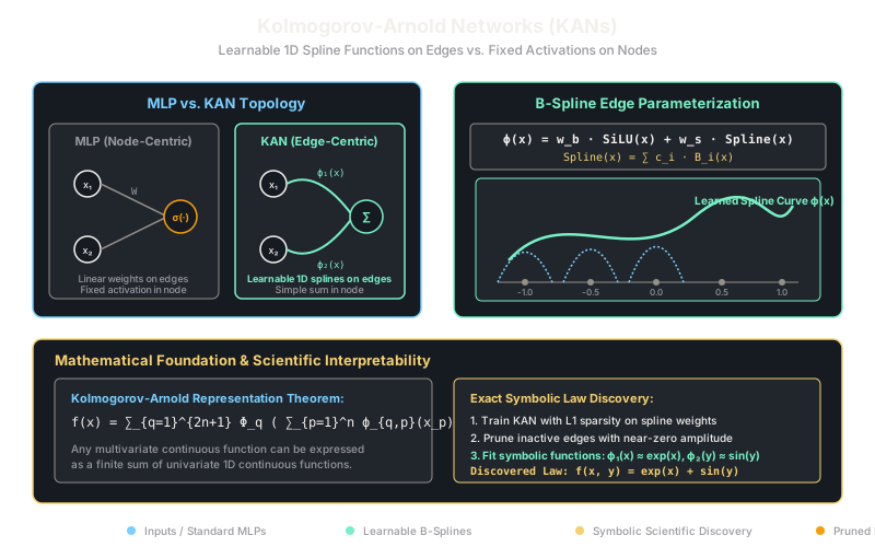
Kolmogorov-Arnold Networks (KANs) flip this architecture completely. Inspired by the Kolmogorov-Arnold representation theorem, KANs have no linear weights on edges and no fixed activation functions on nodes. Instead, the nodes simply compute addition ($\sum$), while the edges carry learnable, univariate B-spline curves.

By placing the non-linear learning mechanism directly on the 1D connections, KANs achieve orders of magnitude lower approximation error on scientific equations, resist catastrophic forgetting, and allow researchers to convert trained neural networks directly into transparent mathematical formulas.

Think of It Like This

How It Actually Works

Splines on Edges, Grid Refinement, and Symbolic Distillation

1. The Kolmogorov-Arnold Representation Theorem

In 1957, mathematicians Andrey Kolmogorov and Vladimir Arnold proved that any multivariate continuous function $f: [0, 1]^n \to \mathbb{R}$ can be expressed as a finite composition of continuous 1D functions and addition:

While Kolmogorov's original theorem established that 2 layers of functions suffice, the original functions $\phi_{q,p}$ could be non-smooth or fractal. Modern KANs generalize this concept into deep arbitrary-depth networks with smooth, differentiable parameterizations.

2. KAN Layer Formulation

A KAN layer with $n_{\text{in}}$ inputs and $n_{\text{out}}$ outputs is defined by a matrix of 1D functions $\mathbf{\Phi} = \{\phi_{q,p}\}$, where $p \in \{1, \dots, n_{\text{in}}\}$ and $q \in \{1, \dots, n_{\text{out}}\}$:

In matrix form: $\mathbf{y} = \mathbf{\Phi}(\mathbf{x})$. A deep KAN network is simply the composition of $L$ such functional layers:

3. B-Spline Parameterization

Each 1D activation function $\phi(x)$ on an edge is parameterized as the sum of a smooth residual base function and a flexible linear combination of B-splines:

where:

• The base function $b(x) = \text{SiLU}(x) = \frac{x}{1 + e^{-x}}$ ensures stable gradient flow during early training.
• The spline term is expanded over $G$ local B-spline basis functions of order $k$ (typically cubic, $k=3$) defined across a uniform knot grid $(t_0, t_1, \dots, t_{G+k})$: $$\text{spline}(x) = \sum_{i=1}^{G+k} c_i B_i(x)$$
• The spline coefficients $c_i$ and scaling parameters $w_b, w_s$ are optimized directly via backpropagation.

4. Grid Extension and Symbolic Discovery

KANs introduce two features impossible in MLPs:

• Grid Extension (Coarse-to-Fine Training): One can train a KAN on a coarse knot grid (e.g., $G = 5$ knots) until convergence, and then interpolate the learned splines onto a finer grid ($G = 20$ knots) with zero loss of accuracy. This prevents catastrophic forgetting and allows continuous accuracy scaling without restarting training.
• Symbolic Distillation: By applying $L_1$ regularization to the spline amplitudes, unimportant edges are pruned. The remaining active 1D spline curves are fitted against a library of mathematical primitives (such as $\sin(x), x^2, \exp(x), \sqrt{x}, \log(x)$). A complex deep KAN collapses into an exact, human-readable scientific formula.

Worked Example

Consider a 1-layer KAN taking 2 inputs $(x_1, x_2)$ to produce 1 output $y$:

Let the knot grid for both edges be defined on $[-1.0, 0.0, 1.0]$ with 3 linear B-spline hat basis functions ($k=1$):

• $B_1(x) = \max(0, 1 - |x - (-1.0)| / 1.0)$ (centered at $-1.0$)
• $B_2(x) = \max(0, 1 - |x - 0.0| / 1.0)$ (centered at $0.0$)
• $B_3(x) = \max(0, 1 - |x - 1.0| / 1.0)$ (centered at $1.0$)

Suppose optimization yields the following spline coefficients ($w_b = 0, w_s = 1$):

• Edge 1 coefficients: $\mathbf{c}^{(1)} = [1.0, 0.0, 1.0]$ (approximating a parabolic curve $x^2$)
• Edge 2 coefficients: $\mathbf{c}^{(2)} = [-1.0, 0.0, 1.0]$ (approximating an identity line $x$)

Now evaluate input $\mathbf{x} = (0.5, -0.4)$:

Evaluate Edge 1 at $x_1 = 0.5$:

$x_1$ lies in the interval $[0.0, 1.0]$:

Spline output:

Evaluate Edge 2 at $x_2 = -0.4$:

$x_2$ lies in the interval $[-1.0, 0.0]$:

Spline output:

Summation at Node:

The network computed the combined non-linear transformation directly through piecewise spline interpolation on each edge.

Code

The following script implements a standalone, vectorized 1D B-spline basis expansion and a single KAN functional layer in PyTorch:

1import torch2import torch.nn as nn3
4
5class LinearBSplineBasis(nn.Module):6    """Linear B-spline basis expansion over a uniform 1D grid."""7
8    def __init__(self, num_knots: int = 5, v_min: float = -1.0, v_max: float = 1.0):9        super().__init__()10        self.knots = torch.linspace(v_min, v_max, num_knots)11        self.step = (v_max - v_min) / (num_knots - 1)12
13    def forward(self, x: torch.Tensor) -> torch.Tensor:14        # x: (Batch, In_Dim) -> returns: (Batch, In_Dim, Num_Knots)15        x_exp = x.unsqueeze(-1)16        # Triangular hat basis: max(0, 1 - |x - knot| / step)17        basis = torch.clamp(1.0 - torch.abs(x_exp - self.knots) / self.step, min=0.0)18        return basis19
20
21class KANLayer(nn.Module):22    """Single KAN layer with learnable spline coefficients on edges."""23
24    def __init__(self, in_features: int, out_features: int, num_knots: int = 5):25        super().__init__()26        self.in_features = in_features27        self.out_features = out_features28        self.spline_basis = LinearBSplineBasis(num_knots=num_knots)29        # Learnable spline coefficients: (out, in, knots)30        self.coefficients = nn.Parameter(31            torch.randn(out_features, in_features, num_knots) * 0.132        )33
34    def forward(self, x: torch.Tensor) -> torch.Tensor:35        # basis: (Batch, In_Dim, Num_Knots)36        basis = self.spline_basis(x)37        # Evaluate each edge spline: sum over knots38        # output: (Batch, Out_Dim)39        spline_vals = torch.einsum("bik,oik->bo", basis, self.coefficients)40        return spline_vals41
42
43# Seed and test with 2 inputs, 1 output44torch.manual_seed(42)45kan = KANLayer(in_features=2, out_features=1, num_knots=5)46
47test_input = torch.tensor([[0.5, -0.4], [0.0, 0.0]], dtype=torch.float32)48output = kan(test_input)49
50print(f"Input coordinates:\n{test_input.numpy()}")51print(f"KAN outputs: {output.detach().numpy().round(4).flatten()}")52# -> Input coordinates:53# -> [[ 0.5 -0.4]54# ->  [ 0.   0. ]]55# -> KAN outputs: [-0.0157  0.0354]

Watch Out For

The Quick Version

• Kolmogorov-Arnold Networks replace linear weights on edges with learnable 1D B-spline curves.
• Network nodes compute simple addition, eliminating fixed node activation functions (like ReLU or GELU).
• KANs scale favorably on scientific function approximation, avoiding the curse of dimensionality seen in MLPs.
• Coarse-to-fine grid extension allows increasing spline resolution without retraining from scratch.
• Pruned KANs can be fitted directly to closed-form symbolic formulas, rendering the model fully interpretable.

What to Read Next

• Domain Adaptation & Generalization
• S4: Structured State Spaces
• Gradient Descent