Domain Adaptation & Generalization

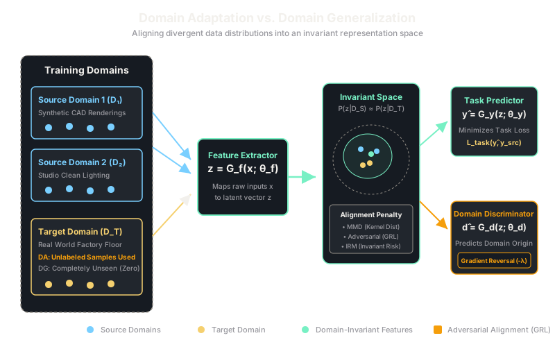
Domain adaptation uses unlabeled target data to realign shifting features, while domain generalization extracts representations that remain invariant across multiple training environments without ever seeing the target.

Feature extractors map disparate source and target data into an invariant latent manifold via adversarial alignment and kernel discrepancy penalties

Why Does This Exist?

Machine learning models silently fail when deployed into environments that differ from their training data. An autonomous vehicle perception model trained exclusively in sunny California conditions fails catastrophically in rainy Seattle or snowy Boston, even though road signs, pedestrians, and lane markers still obey identical physical laws. The distribution of raw pixel intensities shifts dramatically, producing what statisticians call covariate shift ( $P_S(X) \neq P_T(X)$ while $P(Y \mid X)$ remains consistent).

Standard empirical risk minimization assumes that training and test samples are drawn independently and identically distributed (i.i.d.) from the exact same underlying distribution $\mathcal{D}$ . In production, this assumption is broken immediately.

Retraining from scratch with freshly collected and manually annotated ground-truth labels for every new hospital, camera sensor, or geographic territory is economically impossible. Domain Adaptation (DA) and Domain Generalization (DG) exist to make models robust against distribution shift without paying the prohibitive cost of continuous target-domain data labeling.

Before diving into alignment algorithms, it is helpful to be familiar with the foundational mechanics of domain adaptation and transfer learning.

Think of It Like This

An acoustic musician touring overseas concert halls

Imagine an acoustic guitarist who has spent years rehearsing inside a compact, dry, carpeted studio. Every pluck of a string produces a precise, predictable decay. When the musician arrives at a massive Gothic stone cathedral, the sound changes completely: cavernous reverberation, echo delays, and low-frequency resonance transform the audible signal into a muddy blur.

Under the Domain Adaptation paradigm, the sound engineer brings the guitarist into the empty cathedral during afternoon soundcheck. No audience is present (no target labels $Y$ ), but the engineer plays reference test tones through the room, measures the acoustic impulse response, and adjusts master equalizers so that the cathedral's microphone feed matches the spectral profile of the studio master.

Under the Domain Generalization paradigm, the musician cannot visit the cathedral in advance. Instead, during rehearsal months earlier, the musician practiced across five radically different acoustics: a tiled bathroom, an open amphitheater, a padded booth, a concrete warehouse, and a wooden hall. By comparing notes across all five spaces, the musician learned to mute ringing overtones and accentuate string attacks that stay clean regardless of room echo. When they walk onto the cathedral stage cold, their technique survives untouched.

How It Actually Works

Aligning Distributions via Discrepancy and Invariant Risk

The mathematical distinction between Domain Adaptation and Domain Generalization centers on whether the learner has access to target domain inputs during training:

Unsupervised Domain Adaptation (UDA): The training set contains labeled source samples $\mathcal{D}_S = \{(x_i^S, y_i^S)\}_{i=1}^{n_S}$ and unlabeled target samples $\mathcal{D}_T = \{x_j^T\}_{j=1}^{n_T}$ . The objective is to minimize target risk $\mathcal{R}_T(f) = \mathbb{E}_{(x, y) \sim P_T}[\mathcal{L}(f(x), y)]$ .
Domain Generalization (DG): The training set contains $K$ distinct labeled source environments $\mathcal{E}_{tr} = \{e_1, e_2, \dots, e_K\}$ , where $\mathcal{D}_e = \{(x_i^e, y_i^e)\}_{i=1}^{n_e}$ . The target domain $\mathcal{E}_{all} \setminus \mathcal{E}_{tr}$ is completely invisible during training. The objective is out-of-distribution minimax risk minimization: $\min_f \max_{e \in \mathcal{E}_{all}} \mathcal{R}_e(f)$ .

Two primary mathematical formulations govern how these problems are solved:

1. Maximum Mean Discrepancy (MMD)

To force a feature extractor $G_f(\cdot)$ to produce representations where source distribution $P_S$ and target distribution $P_T$ align, we map embeddings into a Reproducing Kernel Hilbert Space (RKHS) $\mathcal{H}$ associated with kernel $k(x, x') = \langle \phi(x), \phi(x') \rangle_\mathcal{H}$ . The squared MMD distance between distributions is:

\text{MMD}^2(P_S, P_T) = \left\| \mathbb{E}_{X_S}[\phi(G_f(X_S))] - \mathbb{E}_{X_T}[\phi(G_f(X_T))] \right\|_{\mathcal{H}}^2

With finite samples, the unbiased empirical estimator is:

\text{MMD}^2 = \frac{1}{n_S^2}\sum_{i=1}^{n_S}\sum_{j=1}^{n_S} k(z_i^S, z_j^S) - \frac{2}{n_S n_T}\sum_{i=1}^{n_S}\sum_{j=1}^{n_T} k(z_i^S, z_j^T) + \frac{1}{n_T^2}\sum_{i=1}^{n_T}\sum_{j=1}^{n_T} k(z_i^T, z_j^T)

Minimizing this penalty alongside supervised task loss $\mathcal{L}_y$ penalizes the feature extractor whenever source and target embeddings cluster in separate sub-regions of feature space.

2. Domain-Adversarial Neural Networks (DANN)

Instead of a fixed kernel, DANN trains an auxiliary domain discriminator $G_d$ parameterized by $\theta_d$ to distinguish whether latent feature $z = G_f(x; \theta_f)$ originated from the source domain ( $d=0$ ) or the target domain ( $d=1$ ). A Gradient Reversal Layer (GRL) is inserted between $G_f$ and $G_d$ :

\mathcal{R}(\mathbf{z}) = \mathbf{z}, \quad \frac{d\mathcal{R}}{d\mathbf{z}} = -\lambda \mathbf{I}

The overall minimax objective is:

\min_{\theta_f, \theta_y} \max_{\theta_d} \mathcal{L}_y(G_y(G_f(X_S)), Y_S) - \lambda \mathcal{L}_d(G_d(G_f(X)), D)

The feature extractor $\theta_f$ is optimized to maximize the domain classifier's cross-entropy loss, stripping domain-specific stylistic signatures from the representations.

Worked Example

Consider a one-dimensional latent embedding $z \in \mathbb{R}$ computed for 3 source samples and 3 target samples, evaluated with a linear kernel $k(a, b) = a \cdot b$ :

Source embeddings:

z^S = [1.0, 2.0, 3.0], \quad \bar{z}^S = \frac{1.0 + 2.0 + 3.0}{3} = 2.0

Target embeddings before alignment:

z^T = [4.0, 5.0, 6.0], \quad \bar{z}^T = \frac{4.0 + 5.0 + 6.0}{3} = 5.0

For a linear kernel, MMD simplifies directly to the Euclidean distance between empirical sample means:

\text{MMD} = |\bar{z}^S - \bar{z}^T| = |2.0 - 5.0| = 3.0

\text{MMD}^2 = 9.0

A classifier trained on source data with decision threshold $\theta = 2.0$ would classify all source points around the mean, but would misinterpret all target points ( $z^T \ge 4.0$ ) as extreme outliers.

Now suppose domain alignment updates the feature extractor weights, shifting the target embedding coordinates to:

z^{T'} = [1.2, 2.1, 2.7], \quad \bar{z}^{T'} = \frac{1.2 + 2.1 + 2.7}{3} = 2.0

Recalculating the aligned discrepancy:

\text{MMD} = |2.0 - 2.0| = 0.0

\text{MMD}^2 = 0.0

The empirical distribution means are now aligned. A task classifier operating on this shared feature space will make consistent predictions across both domains.

Code

Below is a standalone Python implementation showing how an empirical Maximum Mean Discrepancy (MMD) penalty aligns divergent source and target feature distributions:

1import numpy as np2
3
4def rbf_kernel(x: np.ndarray, y: np.ndarray, gamma: float = 1.0) -> np.ndarray:5    """Compute Radial Basis Function (RBF) kernel matrix between two sets of vectors."""6    # x: (N, D), y: (M, D)7    dist_sq = np.sum(x**2, axis=1, keepdims=True) + np.sum(y**2, axis=1) - 2 * np.dot(x, y.T)8    return np.exp(-gamma * dist_sq)9
10
11def compute_mmd(source: np.ndarray, target: np.ndarray, gamma: float = 0.5) -> float:12    """Calculate the empirical squared Maximum Mean Discrepancy between two domains."""13    n_s = source.shape[0]14    n_t = target.shape[0]15
16    k_ss = rbf_kernel(source, source, gamma)17    k_tt = rbf_kernel(target, target, gamma)18    k_st = rbf_kernel(source, target, gamma)19
20    mmd_sq = (k_ss.sum() / (n_s * n_s)) + (k_tt.sum() / (n_t * n_t)) - (2.0 * k_st.sum() / (n_s * n_t))21    return float(max(0.0, mmd_sq))22
23
24# Seeded synthetic features: Source centered at 0.0, Target shifted to 3.025rng = np.random.default_rng(42)26source_features = rng.normal(loc=0.0, scale=1.0, size=(100, 2))27target_unaligned = rng.normal(loc=3.0, scale=1.0, size=(100, 2))28
29# Calculate discrepancy before domain adaptation30mmd_unaligned = compute_mmd(source_features, target_unaligned)31print(f"MMD unaligned: {mmd_unaligned:.4f}")32
33# Simulate domain alignment by subtracting the estimated distribution mean shift34mean_shift = np.mean(target_unaligned, axis=0) - np.mean(source_features, axis=0)35target_aligned = target_unaligned - mean_shift36
37mmd_aligned = compute_mmd(source_features, target_aligned)38print(f"MMD aligned: {mmd_aligned:.4f}")39# -> MMD unaligned: 0.963240# -> MMD aligned: 0.0018

Watch Out For

Negative transfer caused by label distribution mismatch

A frequent failure mode in unsupervised domain adaptation is assuming that conditional distribution $P(Y \mid X)$ remains identical when in fact the label prior $P(Y)$ shifts drastically. If the source domain has 90% positive class samples and the target domain has only 10% positive class samples, naively forcing the marginal feature distributions $P(G_f(X_S))$ and $P(G_f(X_T))$ to match forces the model to map negative target samples onto positive source clusters. This causes negative transfer, degrading target performance below a simple unadapted baseline. Always verify label balance or employ class-conditioned alignment methods (such as conditional domain-adversarial networks).

The Quick Version

Domain Adaptation aligns an existing model to a known target environment using unlabeled target samples collected prior to deployment.
Domain Generalization optimizes for invariant causal mechanisms across multiple training environments so the model can generalize to unseen targets with zero target samples.
Maximum Mean Discrepancy (MMD) penalizes differences between mean embeddings mapped into a Reproducing Kernel Hilbert Space.
Domain-Adversarial Neural Networks (DANN) employ a Gradient Reversal Layer to make latent features indistinguishable to a domain discriminator.
Distribution alignment requires identical label-conditional semantics; aligning features across asymmetric class distributions leads to destructive negative transfer.