Time Series and Forecasting Fundamentals

Time series data records measurements ordered sequentially across time, where the future depends on patterns from the past. Building reliable forecasts requires teasing apart underlying trends, repeating cycles, and noise while strictly preventing future data from leaking into past training steps.

Core time series forecasting workflow detailing trend-seasonal decomposition, weak stationarity properties, autocorrelation function, and rolling-window cross-validation

Why Does This Exist?

Standard supervised machine learning assumes observations are independently and identically distributed ( $i.i.d.$ ). In tabular classification or image processing, shuffling rows or swapping dataset order has zero impact on the mathematical validity of the model.

Time series data violently breaks the $i.i.d.$ assumption. In sequential temporal measurements—such as electricity grid load, server CPU utilization, financial asset prices, or retail product demand—an observation at time $t$ is strongly correlated with observations at $t-1, t-2$ , and $t-k$ . Applying standard machine learning techniques out of the box leads to catastrophic pitfalls:

Temporal Data Leakage: Running random $K$ -fold cross-validation trains the model on future observations (e.g., $t=50$ ) to predict past observations (e.g., $t=20$ ). This produces deceptively stellar validation scores that instantly collapse when deployed to real production environments.
Spurious Regressions from Non-Stationarity: Regressing two unrelated time series that both exhibit an upward secular trend (such as global average temperature versus municipal server counts) yields statistically significant $R^2$ values exceeding $0.95$ despite zero causal or predictive relationship.

Robust time series forecasting requires structuring problems around temporal dependencies: decomposing trends and cycles, enforcing stationarity through differencing, analyzing autocorrelation, and validating strictly using rolling-origin expanding windows.

Think of It Like This

Predicting tomorrow's temperature on an orbiting space station

Imagine you live in a space station rotating once every 24 hours while gradually drifting closer to a star over several months. If you want to forecast tomorrow's temperature, your thermometer reading is not a random draw.

It is the sum of three distinct physical influences:

A slow, persistent trend (the station creeping closer to the star).
A predictable, repeating seasonal cycle (the 24-hour day/night thermal rotation).
Random noise (unpredictable solar flares or air-filter turbulence).

If you want to test whether your forecast algorithm works, you can only give it data from the first two months and ask it to predict the third month. Testing it by giving it random days from month three to predict days in month one is cheating—in real life, tomorrow's sunrise never happens yesterday.

How It Actually Works

Decomposition, Stationarity, and Rolling Horizons

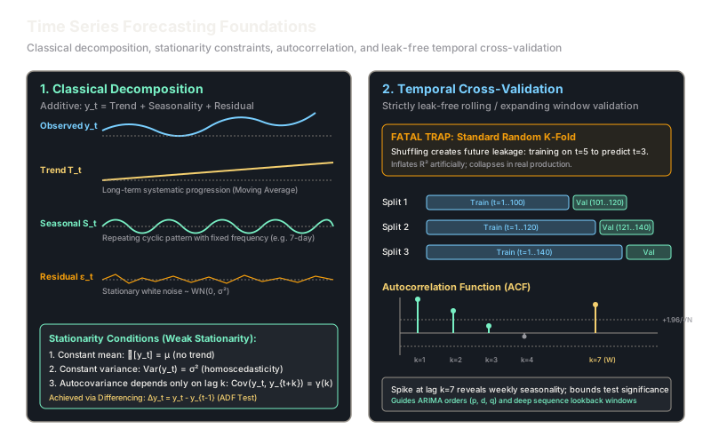
1. Classical Decomposition

A raw univariate time series $y_t$ is modeled as a combination of three structural components:

y_t = f(T_t, S_t, \epsilon_t)

Additive Decomposition: Used when the amplitude of seasonal fluctuations remains constant regardless of the series level: $y_t = T_t + S_t + \epsilon_t$
Multiplicative Decomposition: Used when the seasonal variation scales proportionally with the trend: $y_t = T_t \times S_t \times \epsilon_t \iff \log(y_t) = \log(T_t) + \log(S_t) + \log(\epsilon_t)$

The trend-cycle $T_t$ is estimated using a centered moving average of window size equal to the seasonal period $m$ . The de-trended series $y_t - T_t$ is averaged across repeating periods to isolate $S_t$ , leaving stationary residual noise $\epsilon_t \sim \mathcal{N}(0, \sigma^2)$ .

2. Stationarity and Differencing

A time series is weakly stationary (wide-sense stationary) if its statistical properties do not change over time:

Constant Mean: $\mathbb{E}[y_t] = \mu$ for all $t$ .
Constant Variance: $\operatorname{Var}(y_t) = \sigma^2 < \infty$ for all $t$ .
Time-Invariant Autocovariance: $\operatorname{Cov}(y_t, y_{t+k}) = \gamma(k)$ , depending solely on the temporal lag $k$ , not on the calendar index $t$ .

Non-stationary series containing deterministic or stochastic trends are made stationary through differencing:

\Delta y_t = y_t - y_{t-1}

If a seasonal pattern with period $m$ exists (e.g., 7 days for daily data), seasonal differencing removes it:

\Delta_m y_t = y_t - y_{t-m}

Stationarity is verified statistically using unit root tests such as the Augmented Dickey-Fuller (ADF) test, which tests the null hypothesis $H_0$ that a unit root is present ( $\phi = 1$ in $y_t = \phi y_{t-1} + \epsilon_t$ ). A $p$ -value $< 0.05$ rejects the unit root, confirming stationarity.

3. Autocorrelation Function (ACF) and Partial Autocorrelation (PACF)

The sample autocorrelation at lag $k$ measures the linear correlation between observations $k$ steps apart:

r_k = \frac{\sum_{t=k+1}^T (y_t - \bar{y})(y_{t-k} - \bar{y})}{\sum_{t=1}^T (y_t - \bar{y})^2}

Values outside the Bartlett confidence bands $\pm \frac{1.96}{\sqrt{T}}$ are statistically significant ( $p < 0.05$ ). Spikes at lag $k$ reveal periodic seasonal cycles and indicate the order $p$ and $q$ for autoregressive moving-average (ARIMA) models or the optimal lookback window for deep recurrent networks.

4. Leak-Free Rolling-Origin Cross-Validation

Because temporal sequence is unidirectional, standard random cross-validation leaks information. Instead, practitioners use rolling-origin (expanding window) evaluation:

Fold 1: Train on $[t_1, t_M]$ , test on forecast horizon $[t_{M+1}, t_{M+H}]$ .
Fold 2: Train on $[t_1, t_{M+H}]$ , test on forecast horizon $[t_{M+H+1}, t_{M+2H}]$ .
Fold 3: Train on $[t_1, t_{M+2H}]$ , test on forecast horizon $[t_{M+2H+1}, t_{M+3H}]$ .

Forecast accuracy across horizons $H$ is measured via scale-independent metrics such as Mean Absolute Scaled Error (MASE) or Symmetric Mean Absolute Percentage Error (sMAPE):

\text{MASE} = \frac{\frac{1}{H} \sum_{h=1}^H |y_{T+h} - \hat{y}_{T+h}|}{\frac{1}{T-1} \sum_{t=2}^T |y_t - y_{t-1}|}

A MASE $< 1.0$ proves the model outperforms a naive persistence baseline (predicting $\hat{y}_{T+h} = y_T$ ).

Worked Example

Let us trace autocorrelation and first-order differencing on a 6-day traffic sequence: $y = [100.0, 105.0, 112.0, 120.0, 129.0, 139.0]$

Calculate Sample Mean $\bar{y}$ : $\bar{y} = \frac{100.0 + 105.0 + 112.0 + 120.0 + 129.0 + 139.0}{6} = \frac{705.0}{6} = 117.5$
Compute Total Variance Sum of Squared Deviations (Denominator):
- $t=1: (100.0 - 117.5)^2 = (-17.5)^2 = 306.25$
- $t=2: (105.0 - 117.5)^2 = (-12.5)^2 = 156.25$
- $t=3: (112.0 - 117.5)^2 = (-5.5)^2 = 30.25$
- $t=4: (120.0 - 117.5)^2 = (2.5)^2 = 6.25$
- $t=5: (129.0 - 117.5)^2 = (11.5)^2 = 132.25$
- $t=6: (139.0 - 117.5)^2 = (21.5)^2 = 462.25$ $\sum_{t=1}^6 (y_t - \bar{y})^2 = 306.25 + 156.25 + 30.25 + 6.25 + 132.25 + 462.25 = 1093.50$
Compute Lag-1 Covariance (Numerator for $k=1$ ):
- $t=2: (y_2 - \bar{y})(y_1 - \bar{y}) = (-12.5) \times (-17.5) = 218.75$
- $t=3: (y_3 - \bar{y})(y_2 - \bar{y}) = (-5.5) \times (-12.5) = 68.75$
- $t=4: (y_4 - \bar{y})(y_3 - \bar{y}) = (2.5) \times (-5.5) = -13.75$
- $t=5: (y_5 - \bar{y})(y_4 - \bar{y}) = (11.5) \times (2.5) = 28.75$
- $t=6: (y_6 - \bar{y})(y_5 - \bar{y}) = (21.5) \times (11.5) = 247.25$ $\text{Sum} = 218.75 + 68.75 - 13.75 + 28.75 + 247.25 = 549.75$
Calculate Autocorrelation $r_1$ : $r_1 = \frac{549.75}{1093.50} \approx 0.5027$ A high positive value ( $0.5027$ ) reflects the persistent upward trend.
Apply First Differencing: $\Delta y = [105.0 - 100.0, 112.0 - 105.0, 120.0 - 112.0, 129.0 - 120.0, 139.0 - 129.0] = [5.0, 7.0, 8.0, 9.0, 10.0]$ Differencing eliminates the level shift, converting the raw values into stabilized incremental step rates.

Code

1from typing import List, Tuple2
3def compute_acf(series: List[float], max_lag: int) -> List[float]:4    """Computes sample autocorrelation function (ACF) up to max_lag."""5    n = len(series)6    mean_val = sum(series) / n7    denom = sum((x - mean_val) ** 2 for x in series)8    if denom == 0.0:9        return [1.0] + [0.0] * max_lag10
11    acf_values = [1.0]  # Lag 0 is always 1.012    for k in range(1, max_lag + 1):13        num = sum((series[t] - mean_val) * (series[t - k] - mean_val) for t in range(k, n))14        acf_values.append(num / denom)15    return acf_values16
17
18def difference_series(series: List[float], lag: int = 1) -> List[float]:19    """Calculates lag-k differencing to remove trend or seasonality."""20    return [series[i] - series[i - lag] for i in range(lag, len(series))]21
22
23def rolling_window_split(24    total_len: int, 25    initial_train: int, 26    horizon: int27) -> List[Tuple[Tuple[int, int], Tuple[int, int]]]:28    """Generates strictly leak-free expanding window train/test index bounds."""29    splits = []30    current_end = initial_train31    while current_end + horizon <= total_len:32        train_bounds = (0, current_end)33        test_bounds = (current_end, current_end + horizon)34        splits.append((train_bounds, test_bounds))35        current_end += horizon36    return splits37
38
39raw_data = [100.0, 105.0, 112.0, 120.0, 129.0, 139.0]40acf_vals = compute_acf(raw_data, max_lag=2)41diff_data = difference_series(raw_data, lag=1)42
43print("ACF lags [0, 1, 2]:", [round(v, 4) for v in acf_vals])44# -> ACF lags [0, 1, 2]: [1.0, 0.5027, 0.1065]45print("Differenced series:", diff_data)46# -> Differenced series: [5.0, 7.0, 8.0, 9.0, 10.0]47
48# Expanding window CV across 10 steps with train=6, horizon=249folds = rolling_window_split(total_len=10, initial_train=6, horizon=2)50for idx, (tr, te) in enumerate(folds, 1):51    print(f"Fold {idx}: Train indices {tr}, Test indices {te}")52# -> Fold 1: Train indices (0, 6), Test indices (6, 8)53# -> Fold 2: Train indices (0, 8), Test indices (8, 10)

Watch Out For

Future target leakage via global feature scaling and standardizers

Symptom: An XGBoost or LSTM forecasting pipeline yields near-zero test error in cross-validation, but error surges by $400\%$ when deployed live.

This silent bug occurs when StandardScaler().fit_transform(X) or MinMaxScaler() is executed over the full dataset before splitting into train and test sets. Fitting scalers globally leaks the future minimum, maximum, mean, and standard deviation into historical training steps. Similarly, creating rolling window features (like a 7-day rolling mean) without setting shift(1) causes the target value at $t$ to leak into the feature vector for time $t$ .

Always fit all preprocessors, scalers, imputers, and encoders strictly on the training fold slice, then call transform() on the validation/test horizons. Ensure every lagged feature strictly references $t-1$ or earlier: df['lag_1'] = df['y'].shift(1).

The Quick Version

Time series data breaks the $i.i.d.$ assumption due to strong temporal autocorrelation and chronological ordering.
Classical decomposition separates series into trend-cycle $T_t$ , repeating seasonal cycle $S_t$ , and residual noise $\epsilon_t$ .
Weak stationarity requires constant mean, constant variance, and autocovariance that depends only on the temporal lag.
Differencing $\Delta y_t = y_t - y_{t-1}$ stabilizes non-stationary means and removes secular polynomial trends.
Never use random $K$ -fold cross-validation; always use expanding rolling-origin splits to prevent temporal leakage.