Denoising Diffusion Implicit Models (DDIM)

By generalizing diffusion to a non-Markovian forward process, generation becomes a deterministic trajectory that cuts sampling steps by twenty-fold.

DDIM turns stochastic diffusion into a deterministic ordinary differential equation, enabling 20x faster inference and exact latent space inversion.

Why Does This Exist?

Standard Denoising Diffusion Probabilistic Models (DDPM) unlocked unprecedented visual fidelity, but they suffered from an crippling operational bottleneck: inference latency. Because DDPM defines its reverse generation process as a discrete Markov chain, generating a single image requires sequentially evaluating the denoising U-Net for $T = 1,000$ steps. On a high-end GPU, generating one image took between 10 and 30 seconds.

Furthermore, because DDPM injects independent Gaussian noise at every single reverse step ( $z_t \sim \mathcal{N}(0, I)$ ), the trajectory is strictly stochastic. If a user feeds an existing photograph into the model, there is no deterministic path to invert the photograph back into a unique latent noise representation. Without an invertible latent space, tasks like deterministic image editing, semantic feature blending, and latent-space interpolation become impossible.

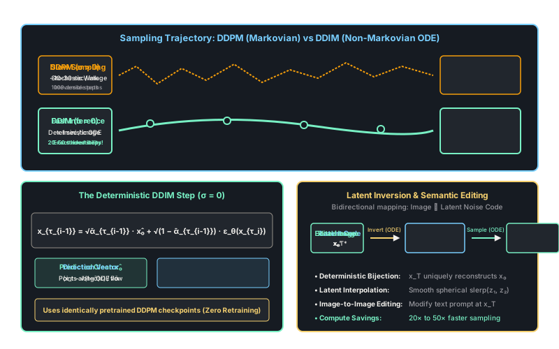
Denoising Diffusion Implicit Models (DDIM) (Song et al., 2020) resolved both problems with a profound theoretical insight: the forward noising process does not need to be Markovian to share the exact same marginal distributions $q(x_t \mid x_0)$ as DDPM. By designing a non-Markovian forward process parameterized by a stochasticity coefficient $\sigma_t$ , setting $\sigma_t = 0$ converts the generation trajectory into a deterministic Ordinary Differential Equation (ODE).

This deterministic formulation allows inference to skip 95% of steps—generating high-fidelity images in just 20 to 50 steps using the exact same pretrained DDPM weights with zero retraining—while establishing a bidirectional bijection between images and noise vectors. Conceptual continuity builds directly upon diffusion-score-based-models.

Think of It Like This

A mountain descent: drifting through a fog versus driving along surveyed contour lines

Imagine descending from the summit of a mountain ( $x_T$ , pure noise) to a specific village in the valley ( $x_0$ , a clean image).

DDPM is like a hiker walking downhill through thick fog. At every single meter of the descent, the hiker checks a compass for general direction, but then stumbles and takes a random sideways step driven by mountain wind (stochastic noise $\sigma_t z$ ). Because there are 1,000 random gusts of wind along the descent, the hiker must take tiny, cautious steps to avoid falling off a cliff. If the hiker reaches a village and tries to climb back up to the exact same summit spot, the random wind makes tracing the path in reverse completely impossible.

DDIM is like a highway engineer paving a paved, banked road down the mountain along the smooth contour lines of the terrain ( $\sigma_t = 0$ ). Because the road follows a continuous, smooth differential curve, you don't need to stop every meter: you can set your cruise control and check your navigation at only 20 milestones along the descent. Even better, because the road is paved and deterministic, you can turn your car around at the valley, drive up the exact same highway in reverse, and arrive at the exact unique parking spot on the summit.

How It Actually Works

Non-Markovian Forward Processes and the Deterministic Reverse Step

In standard DDPM, the forward distribution is strictly Markovian: $q(x_t \mid x_{t-1}, x_0) = q(x_t \mid x_{t-1})$ . DDIM generalizes this by considering a family of non-Markovian forward distributions $q_\sigma(x_{1:T} \mid x_0)$ that satisfy two critical conditions:

The marginal distribution at every step remains identical to DDPM: $q_\sigma(x_t \mid x_0) = \mathcal{N}\left(x_t;\, \sqrt{\bar{\alpha}_t} x_0,\, (1 - \bar{\alpha}_t) I\right)$
The joint distribution conditions on both the previous state and the clean origin $x_0$ : $q_\sigma(x_{t-1} \mid x_t, x_0) = \mathcal{N}\left(x_{t-1};\, \mu(x_t, x_0),\, \sigma_t^2 I\right)$

Because the marginals $q(x_t \mid x_0)$ are identical to DDPM, the objective function $\mathcal{L}_{\text{simple}}(\theta) = \mathbb{E}[\|\epsilon - \epsilon_\theta(x_t, t)\|^2]$ is also identical. Any neural network trained for DDPM can be evaluated with DDIM sampling with zero modification.

The general reverse step equation from timestep $t$ to $t-1$ (or along an arbitrary sub-sequence $\tau_i$ to $\tau_{i-1}$ ) is:

$x_{\tau_{i-1}} = \sqrt{\bar{\alpha}_{\tau_{i-1}}} \underbrace{\left(\frac{x_{\tau_i} - \sqrt{1 - \bar{\alpha}_{\tau_i}}\,\epsilon_\theta(x_{\tau_i}, \tau_i)}{\sqrt{\bar{\alpha}_{\tau_i}}}\right)}_{\text{Predicted Clean Image } \hat{x}_0(x_{\tau_i})} + \underbrace{\sqrt{1 - \bar{\alpha}_{\tau_{i-1}} - \sigma_{\tau_i}^2} \cdot \epsilon_\theta(x_{\tau_i}, \tau_i)}_{\text{Direction Pointing Toward } x_{\tau_i}} + \underbrace{\sigma_{\tau_i} \epsilon}_{\text{Random Noise}}$

where the stochasticity hyperparameter is defined as:

$\sigma_t = \eta \cdot \sqrt{\frac{1 - \bar{\alpha}_{t-1}}{1 - \bar{\alpha}_t}} \sqrt{1 - \frac{\bar{\alpha}_t}{\bar{\alpha}_{t-1}}}$

Two Critical Regimes of $\eta$ :

When $\eta = 1.0$ : $\sigma_t$ equals the forward posterior variance of DDPM, recovering standard stochastic Markovian diffusion.
When $\eta = 0.0$ : $\sigma_t = 0$ . The random noise term $\sigma_{\tau_i} \epsilon$ vanishes completely!

When $\sigma_t = 0$ , the reverse update becomes a deterministic discretization of the Probability Flow ODE:

$x_{\tau_{i-1}} = \sqrt{\bar{\alpha}_{\tau_{i-1}}} \hat{x}_0(x_{\tau_i}) + \sqrt{1 - \bar{\alpha}_{\tau_{i-1}}} \cdot \epsilon_\theta(x_{\tau_i}, \tau_i)$

Sub-sequence Striding

Because the transition is governed by an ODE rather than a step-by-step Markov chain, we can select an arbitrary strided sub-sequence of timesteps $\tau = [\tau_1, \tau_2, \dots, \tau_S]$ where $S \ll T$ . For example, choosing $S = 50$ steps out of $T = 1,000$ evaluates timesteps $[1, 21, 41, \dots, 981]$ , cutting inference computation by $20\times$ with negligible loss in sample quality.

Worked Example

Let us trace a single deterministic DDIM step ( $\eta = 0, \sigma = 0$ ) jumping from timestep $\tau_i = 100$ down to $\tau_{i-1} = 50$ :

Given schedule parameters:
- At step $100$ : $\bar{\alpha}_{100} = 0.70 \implies \sqrt{\bar{\alpha}_{100}} = \sqrt{0.70} \approx 0.8367$ , $\sqrt{1 - \bar{\alpha}_{100}} = \sqrt{0.30} \approx 0.5477$ .
- At step $50$ : $\bar{\alpha}_{50} = 0.85 \implies \sqrt{\bar{\alpha}_{50}} = \sqrt{0.85} \approx 0.9220$ , $\sqrt{1 - \bar{\alpha}_{50}} = \sqrt{0.15} \approx 0.3873$ .
Current state and model prediction: Suppose current scalar coordinate is $x_{100} = 1.50$ , and the neural network predicts noise $\epsilon_\theta(x_{100}, 100) = 0.60$ .
Step 1: Estimate predicted clean origin $\hat{x}_0$ : $\hat{x}_0 = \frac{x_{100} - \sqrt{1 - \bar{\alpha}_{100}} \cdot \epsilon_\theta}{\sqrt{\bar{\alpha}_{100}}} = \frac{1.50 - 0.5477 \times 0.60}{0.8367} = \frac{1.50 - 0.3286}{0.8367} = \frac{1.1714}{0.8367} \approx 1.400$
Step 2: Compute next deterministic state $x_{50}$ : $x_{50} = \sqrt{\bar{\alpha}_{50}} \cdot \hat{x}_0 + \sqrt{1 - \bar{\alpha}_{50}} \cdot \epsilon_\theta$ $x_{50} = 0.9220 \times 1.400 + 0.3873 \times 0.60 = 1.2908 + 0.2324 = 1.5232$

Notice: Zero random numbers were sampled. The mapping from $x_{100}$ to $x_{50}$ is completely deterministic and exact.

Code

1import torch2
3def ddim_step(4    x_t: torch.Tensor,5    eps_pred: torch.Tensor,6    alpha_bar_t: float,7    alpha_bar_prev: float,8    eta: float = 0.0,9) -> torch.Tensor:10    """Computes a single reverse DDIM step from timestep t to prev_t.11    When eta=0.0, the update is completely deterministic.12    """13    # 1. Predict clean x_0 from current noisy state14    sqrt_alpha_bar_t = alpha_bar_t ** 0.515    sqrt_one_minus_alpha_bar_t = (1.0 - alpha_bar_t) ** 0.516    pred_x0 = (x_t - sqrt_one_minus_alpha_bar_t * eps_pred) / sqrt_alpha_bar_t17    18    # 2. Compute stochastic variance sigma_t19    if eta > 0.0:20        sigma = eta * (21            ((1.0 - alpha_bar_prev) / (1.0 - alpha_bar_t)) ** 0.522            * (1.0 - alpha_bar_t / alpha_bar_prev) ** 0.523        )24    else:25        sigma = 0.026        27    # 3. Direction vector pointing to x_t28    dir_xt = (1.0 - alpha_bar_prev - sigma ** 2) ** 0.5 * eps_pred29    30    # 4. Deterministic next state31    x_prev = (alpha_bar_prev ** 0.5) * pred_x0 + dir_xt32    33    # 5. Add stochastic noise if eta > 034    if sigma > 0.0:35        noise = torch.randn_like(x_t)36        x_prev = x_prev + sigma * noise37        38    return x_prev39
40# Demonstration: Deterministic reproducibility41x_current = torch.tensor([1.50])42eps_model = torch.tensor([0.60])43a_bar_t = 0.7044a_bar_prev = 0.8545
46# Running the function twice with eta=0.0 yields identical tensors47out1 = ddim_step(x_current, eps_model, a_bar_t, a_bar_prev, eta=0.0)48out2 = ddim_step(x_current, eps_model, a_bar_t, a_bar_prev, eta=0.0)49
50print(f"DDIM output: {out1.item():.4f}")51# -> DDIM output: 1.523152print("Exact equality across independent runs:", torch.equal(out1, out2))53# -> Exact equality across independent runs: True

Watch Out For

Accumulated discretization drift during DDIM inversion without null-text guidance matching

Inverting a real image $x_0$ to its latent noise vector $x_T$ via reverse ODE integration relies on local Euler approximations: $\frac{dx}{dt} \approx \frac{x_{t+\Delta t} - x_t}{\Delta t}$ . When running reverse ODE generation from $x_T$ back to $x_0$ , discretization errors compound at each step. If Classifier-Free Guidance (CFG) is enabled during generation, the forward inversion and reverse generation trajectories diverge significantly, resulting in generated images that alter facial identities or structural compositions.

To achieve exact reconstruction in image editing pipelines, perform Null-Text Inversion (Mokady et al., 2023): keep the model guidance scale aligned or optimize the unconditional text embedding vector at each inversion step to guarantee that the reverse ODE trajectory retraces the forward inversion trajectory with near-zero mathematical drift.

The Quick Version

DDIM reformulates the diffusion forward process as non-Markovian, preserving the exact same marginal distributions and training objective as DDPM.
Setting the stochasticity parameter $\eta = 0$ transforms diffusion into a deterministic Probability Flow ODE.
Strided sub-sequence sampling allows generating high-fidelity images in 20 to 50 steps ( $20\times$ faster than DDPM) while enabling exact latent space inversion for image editing.