Diffusion and Score-Based Models

Data is gradually corrupted with Gaussian noise over hundreds of steps, and a neural network learns to reverse the process step by step.

Diffusion models corrupt data with scheduled Gaussian noise, training a neural network to estimate the Stein score and denoise reverse trajectories.

Why Does This Exist?

Prior to diffusion models, generative modeling was split between three flawed paradigms:

Generative Adversarial Networks (GANs): Capable of generating sharp images, but notoriously unstable to train due to adversarial min-max dynamics, hyperparameter sensitivity, and catastrophic mode collapse.
Variational Autoencoders (VAEs): Stable to train via likelihood bounds, but produce blurry images because approximating true posterior distributions with simple Gaussians forces the decoder to average across plausible modes.
Autoregressive Models: Excellent likelihood estimates, but generate images one pixel or token at a time, resulting in severe inference latency.

Diffusion Models (Denoising Diffusion Probabilistic Models, DDPM) and Score-Based Generative Models (SGMs) overcome these limitations by framing generation as reversing a thermodynamic diffusion process. Rather than attempting to map a simple Gaussian distribution directly to complex natural images in a single massive jump, diffusion breaks generation down into hundreds or thousands of tiny, tractable denoising steps.

Training requires no adversarial discriminator; instead, a standard neural network (typically a U-Net) is trained with simple mean squared error to predict the noise injected at an arbitrary timestep. Training is unconditionally stable, covers all modes of the distribution, and achieves state-of-the-art sample quality. Foundation concepts rely on understanding regression loss-functions.

Think of It Like This

A perfume drop dissolving in water filmed in reverse

Imagine releasing a single drop of concentrated purple perfume into a clear glass of water.

In the forward process (diffusion), the concentrated drop naturally expands. Water molecules collide with perfume particles, scattering them randomly. At step 10, the drop is slightly fuzzy. At step 200, purple wisps curl through the liquid. At step 1,000, the glass is completely uniform, faint purple water: maximum entropy, all original structure completely destroyed. Every drop of perfume, regardless of whether it was shaped like a star or a circle, ends up as identical uniform noise.

Now imagine running the film backward. If you know the precise statistical laws governing how water molecules pushed the perfume particles outward, you can nudge every particle slightly inward against the current. By taking 1,000 microscopic reverse steps, you can start from completely random purple water and assemble the scattered molecules back into a pristine, concentrated drop.

How It Actually Works

Forward SDEs, Score Matching, and the DDPM Objective

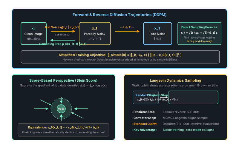
The diffusion framework can be understood through two unified lenses: discrete Markov chains (DDPM) and continuous stochastic differential equations (Score-based models).

1. Discrete Forward Process (DDPM)

Given data $x_0 \sim q(x_0)$ , the forward Markov chain adds Gaussian noise according to a fixed variance schedule $\beta_1, \beta_2, \dots, \beta_T$ :

$q(x_t \mid x_{t-1}) = \mathcal{N}\left(x_t;\, \sqrt{1 - \beta_t} x_{t-1},\, \beta_t I\right)$

A key mathematical property of Gaussian transitions is that we can sample $x_t$ at any arbitrary timestep $t$ in closed form without iterating through intermediate steps. Defining $\alpha_t = 1 - \beta_t$ and $\bar{\alpha}_t = \prod_{s=1}^t \alpha_s$ :

$q(x_t \mid x_0) = \mathcal{N}\left(x_t;\, \sqrt{\bar{\alpha}_t} x_0,\, (1 - \bar{\alpha}_t) I\right)$

$x_t = \sqrt{\bar{\alpha}_t} x_0 + \sqrt{1 - \bar{\alpha}_t} \epsilon, \quad \epsilon \sim \mathcal{N}(0, I)$

2. Reverse Process and Simplified Loss

The reverse process $p_\theta(x_{t-1} \mid x_t)$ is also Gaussian for sufficiently small $\beta_t$ :

$p_\theta(x_{t-1} \mid x_t) = \mathcal{N}\left(x_{t-1};\, \mu_\theta(x_t, t),\, \Sigma_\theta(x_t, t)\right)$

Ho et al. (2020) proved that reparameterizing the mean $\mu_\theta$ to predict the injected noise vector $\epsilon$ yields a simplified variational lower bound objective:

$\mathcal{L}_{\text{simple}}(\theta) = \mathbb{E}_{t \sim U[1, T],\, x_0 \sim q(x_0),\, \epsilon \sim \mathcal{N}(0, I)} \left[ \|\epsilon - \epsilon_\theta(x_t, t)\|_2^2 \right]$

During training, an algorithm:

Samples a clean image $x_0$ and a random timestep $t \in \{1, \dots, T\}$ .
Samples standard normal noise $\epsilon \sim \mathcal{N}(0, I)$ .
Computes noisy image $x_t = \sqrt{\bar{\alpha}_t} x_0 + \sqrt{1 - \bar{\alpha}_t} \epsilon$ .
Passes $x_t$ and timestep embedding $t$ to neural network $\epsilon_\theta$ .
Calculates MSE between true noise $\epsilon$ and predicted noise $\epsilon_\theta(x_t, t)$ .

3. Score-Based Perspective

Song and Ermon (2019) developed generation via the Stein score function, defined as the gradient of the log probability density with respect to the data:

$s(x) \equiv \nabla_x \log p(x)$

The score function is a vector field pointing in the direction where data density increases most rapidly. Score matching trains a neural network $s_\theta(x, \sigma)$ to approximate this gradient without ever calculating the intractable normalizing partition function of $p(x)$ .

The connection between DDPM and Score Matching is exact:

$s_\theta(x_t, t) = -\frac{\epsilon_\theta(x_t, t)}{\sqrt{1 - \bar{\alpha}_t}}$

Sampling is performed using Annealed Langevin Dynamics:

$x_{k+1} = x_k + \frac{\delta}{2} s_\theta(x_k, \sigma_i) + \sqrt{\delta} z_k, \quad z_k \sim \mathcal{N}(0, I)$

Worked Example

Let us trace a single forward corruption and training evaluation step on a 2D toy vector $x_0 = [1.2, -0.8]$ at timestep $t = 500$ :

Schedule parameter values at $t = 500$ : Suppose the cumulative noise factor is $\bar{\alpha}_{500} = 0.64$ . $\sqrt{\bar{\alpha}_{500}} = \sqrt{0.64} = 0.80$ $\sqrt{1 - \bar{\alpha}_{500}} = \sqrt{1 - 0.64} = \sqrt{0.36} = 0.60$
Sample random noise $\epsilon$ : Sample $\epsilon = [0.50, -1.00] \sim \mathcal{N}(0, I)$ .
Compute noisy coordinate $x_{500}$ : $x_{500} = 0.80 \times [1.2, -0.8] + 0.60 \times [0.50, -1.00]$ $= [0.96, -0.64] + [0.30, -0.60] = [1.26, -1.24]$
Model noise prediction and loss: Assume the U-Net evaluates $x_{500}$ and outputs $\hat{\epsilon} = \epsilon_\theta(x_{500}, 500) = [0.45, -0.90]$ . Compute squared error against true noise $\epsilon = [0.50, -1.00]$ : $\mathcal{L} = \frac{1}{2}\left( (0.50 - 0.45)^2 + (-1.00 - (-0.90))^2 \right)$ $= \frac{1}{2}\left( 0.05^2 + (-0.10)^2 \right) = \frac{1}{2}(0.0025 + 0.0100) = 0.00625$
Corresponding score vector estimate: $s_\theta(x_{500}, 500) = -\frac{[0.45, -0.90]}{0.60} = [-0.75, 1.50]$ The score vector points back toward the high-density region where $x_0 = [1.2, -0.8]$ resides!

Code

1import torch2import torch.nn as nn3import torch.nn.functional as F4
5class DiffusionForward:6    """Precomputes closed-form coefficients for forward Gaussian diffusion."""7    def __init__(self, timesteps: int = 1000, beta_start: float = 1e-4, beta_end: float = 0.02):8        self.timesteps = timesteps9        # Linear beta schedule10        self.betas = torch.linspace(beta_start, beta_end, timesteps)11        self.alphas = 1.0 - self.betas12        self.alphas_cumprod = torch.cumprod(self.alphas, dim=0)13        self.sqrt_alphas_cumprod = torch.sqrt(self.alphas_cumprod)14        self.sqrt_one_minus_alphas_cumprod = torch.sqrt(1.0 - self.alphas_cumprod)15
16    def q_sample(self, x_0: torch.Tensor, t: torch.Tensor, noise: torch.Tensor | None = None) -> tuple[torch.Tensor, torch.Tensor]:17        """Closed-form jump to arbitrary timestep t."""18        if noise is None:19            noise = torch.randn_like(x_0)20        21        sqrt_alpha = self.sqrt_alphas_cumprod[t].view(-1, 1, 1, 1)22        sqrt_one_minus_alpha = self.sqrt_one_minus_alphas_cumprod[t].view(-1, 1, 1, 1)23        24        x_t = sqrt_alpha * x_0 + sqrt_one_minus_alpha * noise25        return x_t, noise26
27# Test closed-form forward sampling28diff = DiffusionForward(timesteps=1000)29x_0 = torch.randn(4, 3, 32, 32)30# Sample random timesteps for a batch31t = torch.tensor([50, 250, 500, 900])32x_t, noise = diff.q_sample(x_0, t)33
34print("x_t shape:", x_t.shape)35# -> x_t shape: torch.Size([4, 3, 32, 32])36print("Noise shape:", noise.shape)37# -> Noise shape: torch.Size([4, 3, 32, 32])38
39# Measure variance at t=50 vs t=90040alpha_bar_50 = diff.alphas_cumprod[50].item()41alpha_bar_900 = diff.alphas_cumprod[900].item()42print(f"Signal preserved at t=50: {alpha_bar_50 * 100:.1f}%")43# -> Signal preserved at t=50: 98.4%44print(f"Signal preserved at t=900: {alpha_bar_900 * 100:.1f}%")45# -> Signal preserved at t=900: 0.8%

Watch Out For

Sampling timesteps uniformly without noise schedule variance adjustment

When training on higher-resolution images or using linear beta schedules ( $\beta_1 = 10^{-4}$ to $\beta_T = 0.02$ ), the signal-to-noise ratio drops to near-zero too quickly in the middle of the trajectory. By timestep $t=500$ , virtually all high-frequency details are gone, forcing the network to spend over half its training capacity predicting pure noise without learning structural semantic features.

In modern implementations, switch from a naive linear schedule to a cosine noise schedule (Nichol & Dhariwal, 2021). The cosine schedule ensures that $\bar{\alpha}_t$ drops smoothly following $\cos^2\left(\frac{t/T + s}{1 + s} \cdot \frac{\pi}{2}\right)$ , preserving useful image structural information across a much wider fraction of timesteps and dramatically accelerating convergence.

The Quick Version

Diffusion models decompose generative modeling into hundreds of small denoising steps, eliminating the training instability and mode collapse inherent to GANs.
The forward process adds Gaussian noise according to variance schedule $\beta_t$ , permitting direct closed-form sampling of noisy state $x_t$ at any timestep $t$ .
Training minimizes simple MSE loss between true added noise $\epsilon$ and network prediction $\epsilon_\theta(x_t, t)$ , which is mathematically equivalent to estimating the Stein score $\nabla_x \log p(x)$ .