Latent Diffusion Models

Diffusion is moved out of pixel space into a compressed latent space learned by an autoencoder, cutting compute costs by orders of magnitude while preserving fine detail.

Why Does This Exist?

Early diffusion models like DDPM and score-based models operated directly in pixel space. Generating a photorealistic $512 \times 512$ RGB image requires evaluating a massive neural network over $512 \times 512 \times 3 = 786,432$ distinct numerical coordinates at every single timestep.

Digital images exhibit massive spatial redundancy: neighboring pixels in a blue sky or wooden table share nearly identical values. In pixel-space diffusion, the denoising U-Net spends the vast majority of its floating-point operations (FLOPs) learning high-frequency imperceptible details—such as microscopic noise textures in smooth background surfaces—rather than learning the high-level semantic composition and global layout of the scene.

To train high-resolution models, earlier practitioners were forced to build cumbersome cascades of separate models: a base model generating blurry $64 \times 64$ images, followed by two separate super-resolution diffusion models upscaling to $256 \times 256$ and $1024 \times 1024$ . This cascaded architecture required hundreds of GPU-years to train and made interactive consumer inference impossible.

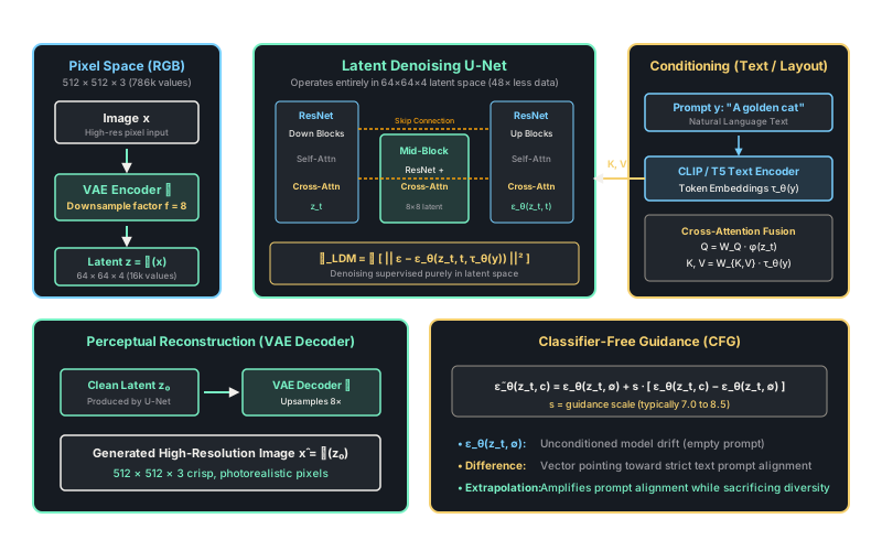
Latent Diffusion Models (LDM) (Rombach et al., 2022)—the foundational breakthrough behind Stable Diffusion—solve this by explicitly decoupling perceptual compression from semantic generation. An autoencoder compresses high-dimensional images into a perceptually equivalent, low-dimensional latent space ( $64\times$ spatial compression). The diffusion model then operates entirely inside this compact latent representation, reducing memory and compute requirements by nearly $50\times$ while enabling flexible conditioning on text, depth maps, and segmentation masks. Prerequisite knowledge connects directly to diffusion-score-based-models.

Think of It Like This

An architect drafting blueprints instead of hauling concrete bricks

Imagine an architect designing a cathedral.

Pixel-space diffusion is like hiring a team of bricklayers to test structural layouts by physically stacking 800,000 full-sized granite bricks on an open construction lot. If the roof looks slightly unbalanced, the crew must dismantle and restack all 800,000 heavy bricks, spending 99% of their physical energy moving stone and only 1% contemplating aesthetic proportion.

Latent diffusion is how modern architecture actually works. An expert draughtsman (the VAE encoder) converts the messy physical site into a clean, compact $1:64$ scale blueprint on a drafting board. The architect (the latent diffusion U-Net) sits at the desk, easily sketching, erasing, and refining the structural arches on the lightweight blueprint without lifting a single stone.

Beside the desk sits a client (the text prompt) providing instructions like "add stained-glass rose windows" (cross-attention). Once the blueprint is perfectly rendered and balanced, a master builder (the VAE decoder) reads the finished blueprint and constructs the real-world stone cathedral in a single pass.

How It Actually Works

Two-Stage Separation and Cross-Attention Conditioning

Latent Diffusion Models divide image synthesis into two distinct stages:

Stage 1: Perceptual Compression (Autoencoder)

A regularized autoencoder trained with perceptual and patch-based adversarial losses consists of an encoder $\mathcal{E}$ and a decoder $\mathcal{D}$ . Given an image $x \in \mathbb{R}^{H \times W \times 3}$ , the encoder compresses it into a latent code $z = \mathcal{E}(x) \in \mathbb{R}^{h \times w \times c}$ , where the downsampling factor is $f = H/h = W/w = 2^m$ . In Stable Diffusion, $f = 8$ , compressing an input of shape $(512, 512, 3)$ into a latent tensor $z$ of shape $(64, 64, 4)$ .

To prevent arbitrarily high-variance latent spaces, the autoencoder is regularized either via a mild Kullback-Leibler penalty toward a standard normal distribution (KL-reg) or via vector quantization (VQ-reg). The decoder reconstructs the image from the latent: $\hat{x} = \mathcal{D}(z) \approx x$ .

Stage 2: Latent Denoising and Conditioning

The diffusion model operates entirely in latent space $\mathcal{Z}$ . The forward process adds Gaussian noise to the clean latent $z_0 = \mathcal{E}(x)$ :

$z_t = \sqrt{\bar{\alpha}_t} z_0 + \sqrt{1 - \bar{\alpha}_t} \epsilon, \quad \epsilon \sim \mathcal{N}(0, I)$

A time-conditional U-Net $\epsilon_\theta(z_t, t, \tau_\theta(y))$ is trained to predict the added noise vector:

$\mathcal{L}_{\text{LDM}}(\theta) = \mathbb{E}_{\mathcal{E}(x),\, y,\, \epsilon \sim \mathcal{N}(0, I),\, t} \left[ \|\epsilon - \epsilon_\theta(z_t, t, \tau_\theta(y))\|_2^2 \right]$

where $y$ is the conditioning input (such as a text prompt), and $\tau_\theta(y) \in \mathbb{R}^{M \times d_\tau}$ is a domain-specific encoder (such as a frozen CLIP ViT-L/14 or T5 text encoder).

Cross-Attention Fusion

The conditioning representation $\tau_\theta(y)$ is injected into the intermediate layers of the U-Net via cross-attention. For an intermediate feature map $\phi_i(z_t) \in \mathbb{R}^{N \times d_\epsilon}$ :

$Q = W_Q^{(i)} \phi_i(z_t), \quad K = W_K^{(i)} \tau_\theta(y), \quad V = W_V^{(i)} \tau_\theta(y)$

$\text{Attention}(Q, K, V) = \text{softmax}\left(\frac{Q K^T}{\sqrt{d_k}}\right) V$

Classifier-Free Guidance (CFG)

To steer generation strongly toward the text prompt, the model is trained with conditional dropout: 10% of training steps drop the prompt $y$ , replacing it with an empty null token $\emptyset$ . During inference, the model evaluates both the unconditioned and conditioned noise predictions:

$\tilde{\epsilon}_\theta(z_t, t, c) = \epsilon_\theta(z_t, t, \emptyset) + s \cdot \left(\epsilon_\theta(z_t, t, c) - \epsilon_\theta(z_t, t, \emptyset)\right)$

where $s \ge 1$ (typically $s \in [7.0, 8.5]$ ) is the guidance scale. Values of $s > 1$ extrapolate away from generic images toward compositions that strictly adhere to the prompt.

Worked Example

Let us examine the data reduction and a concrete Classifier-Free Guidance step:

Dimensional Compression Ratio:
- Pixel image $x$ : $512 \times 512 \times 3 = 786,432$ floats.
- Latent representation $z$ : $64 \times 64 \times 4 = 16,384$ floats.
- Memory and representation reduction: $\frac{786,432}{16,384} = 48\times \text{ reduction in sequence size}$ For self-attention layers with quadratic spatial complexity $\mathcal{O}((H \cdot W)^2)$ , compressing spatial dimensions from $512 \times 512 = 262,144$ tokens to $64 \times 64 = 4,096$ tokens achieves a theoretical $(64)^2 = \mathbf{4,096\times}$ reduction in attention matrix memory!
Classifier-Free Guidance Extrapolation: Suppose at latent pixel coordinate $(12, 34)$ in channel 0:
- Unconditioned noise prediction (empty prompt): $\epsilon_\theta(z_t, \emptyset) = 0.20$
- Conditioned noise prediction ("a red lighthouse"): $\epsilon_\theta(z_t, c) = 0.60$
- Guidance scale: $s = 7.5$
Calculate extrapolated noise update: $\text{Difference} = \epsilon_\theta(z_t, c) - \epsilon_\theta(z_t, \emptyset) = 0.60 - 0.20 = 0.40$ $\tilde{\epsilon} = 0.20 + 7.5 \times (0.40) = 0.20 + 3.00 = 3.20$ The guidance formula amplifies the model's text-aligned direction eight-fold relative to the unconditioned drift.

Code

1import torch2import torch.nn as nn3import torch.nn.functional as F4
5class CrossAttentionBlock(nn.Module):6    """Computes cross-attention between spatial latent features and text embeddings."""7    def __init__(self, query_dim: int = 320, context_dim: int = 768, num_heads: int = 8):8        super().__init__()9        self.num_heads = num_heads10        self.head_dim = query_dim // num_heads11        self.to_q = nn.Linear(query_dim, query_dim, bias=False)12        self.to_k = nn.Linear(context_dim, query_dim, bias=False)13        self.to_v = nn.Linear(context_dim, query_dim, bias=False)14        self.to_out = nn.Linear(query_dim, query_dim)15
16    def forward(self, x: torch.Tensor, context: torch.Tensor) -> torch.Tensor:17        # x: (batch, seq_len_latent, query_dim) e.g., (2, 4096, 320)18        # context: (batch, seq_len_text, context_dim) e.g., (2, 77, 768)19        b, n, _ = x.shape20        q = self.to_q(x).view(b, n, self.num_heads, self.head_dim).transpose(1, 2)21        k = self.to_k(context).view(b, -1, self.num_heads, self.head_dim).transpose(1, 2)22        v = self.to_v(context).view(b, -1, self.num_heads, self.head_dim).transpose(1, 2)23        24        # Scaled dot-product attention25        scores = torch.matmul(q, k.transpose(-2, -1)) / (self.head_dim ** 0.5)26        attn = F.softmax(scores, dim=-1)27        out = torch.matmul(attn, v).transpose(1, 2).contiguous().view(b, n, -1)28        return self.to_out(out)29
30def apply_classifier_free_guidance(31    noise_uncond: torch.Tensor, noise_cond: torch.Tensor, guidance_scale: float32) -> torch.Tensor:33    """Extrapolates noise prediction toward prompt direction."""34    return noise_uncond + guidance_scale * (noise_cond - noise_uncond)35
36# Verification37latent_features = torch.randn(2, 64, 320)      # 64 spatial tokens38text_embeddings = torch.randn(2, 77, 768)      # 77 CLIP tokens39cross_attn = CrossAttentionBlock()40
41output = cross_attn(latent_features, text_embeddings)42print("Conditioned latent feature shape:", output.shape)43# -> Conditioned latent feature shape: torch.Size([2, 64, 320])44
45# CFG Verification46eps_uncond = torch.tensor([0.20, -0.15])47eps_cond = torch.tensor([0.60, -0.45])48guided_eps = apply_classifier_free_guidance(eps_uncond, eps_cond, guidance_scale=7.5)49print("Guided noise vector:", guided_eps.tolist())50# -> Guided noise vector: [3.200000047683716, -2.4000000953674316]

Watch Out For

Latent scaling factor mismatch between VAE encoder and diffusion noise schedule

When an image is passed through a pretrained VAE encoder $z = \mathcal{E}(x)$ , the resulting latent tensor does not naturally have unit variance ( $\sigma^2 \ne 1$ ). In Stable Diffusion v1, the latent codes have an empirical standard deviation of approximately $\sigma \approx 5.5$ .

If you feed these unscaled latents directly into a diffusion model whose noise schedule assumes unit variance inputs ( $\mathcal{N}(0, I)$ ), the added noise at small timesteps is completely overwhelmed by the large variance of the latent code. To fix this, always scale the latent codes by a fixed scaling factor before diffusion: z = z * 0.18215 (and divide by 0.18215 before passing to the VAE decoder). Forgetting this scaling factor destroys image generation, causing the model to output blurry, contrast-saturated noise artifacts.

The Quick Version

Latent Diffusion Models decouple perceptual compression (handled by a pretrained VAE) from semantic generation (handled by a latent U-Net).
Compressing $512 \times 512$ images by an $8\times$ factor into $64 \times 64 \times 4$ latents cuts data volume by $48\times$ and attention computation by over $4,000\times$ .
Text conditioning is injected via cross-attention between latent U-Net features and CLIP text tokens, with Classifier-Free Guidance amplifying adherence to prompts.