S4: Structured State Spaces

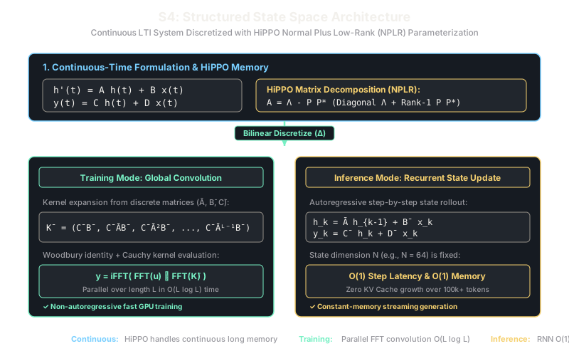
S4 models sequence data by combining the constant-time token generation of recurrent neural networks with the parallelizable convolutional training of transformers.

S4 bridges continuous differential equations and discrete sequence modeling using diagonal-plus-low-rank matrix decomposition

Why Does This Exist?

Sequence modeling has historically been trapped between two opposing trade-offs:

Recurrent Neural Networks (RNNs) process tokens sequentially with $O(1)$ memory and constant step latency during inference, but suffer from vanishing gradients and cannot train in parallel across time steps ( $O(L)$ sequential dependencies).
Transformers parallelize training across sequence length $L$ via dense attention matrices, but their attention mechanism scales quadratically ( $O(L^2)$ computation and memory), and autoregressive inference requires an ever-growing Key-Value cache that exhausts GPU high-bandwidth memory at context lengths exceeding tens of thousands of tokens.

Linear continuous-time State Space Models (SSMs) offer a theoretical path out of this dilemma. By mapping a continuous input signal $x(t)$ through an implicit latent state $h(t) \in \mathbb{R}^N$ , SSMs can be evaluated either as a linear recurrence or as a 1D convolution.

However, standard discrete SSMs collapsed in practice. Computing the convolution kernel $\bar{K} = (C\bar{B}, C\bar{A}\bar{B}, \dots, C\bar{A}^{L-1}\bar{B})$ requires repeatedly multiplying an $N \times N$ transition matrix $\bar{A}$ across sequence length $L$ . Naive matrix powers require $O(N^2 L)$ operations and $O(N L)$ memory per channel. When $N = 64$ and $L = 100{,}000$ , training instantly runs out of memory. Furthermore, random state matrices suffer from exponential memory decay, failing the Long Range Arena benchmark.

Structured State Spaces for Sequence Modeling (S4) solved this bottleneck by introducing the Normal Plus Low-Rank (NPLR) parameterization of the HiPPO memory matrix, reducing kernel computation from quadratic to $O(N + L)$ and unlocking sub-quadratic long-context sequence modeling. Before exploring S4's algebraic machinery, review the fundamentals of general state-space models and transformers.

Think of It Like This

An analog radio receiver with synchronized resonance tuning

Think of an analog AM/FM radio receiver listening to a continuous audio broadcast. The receiver does not store an audio recording of every millisecond that passed since the radio was turned on; storing raw audio samples forever would require infinite magnetic tape.

Instead, the tuner contains a bank of resonant electronic filter circuits (RLC oscillators). Each circuit resonates at a distinct frequency harmonic. As the incoming radio wave hits the antenna, each oscillator continuously vibrates, summarizing the continuous history of the broadcast into a compact set of harmonic coefficients.

The HiPPO matrix in S4 is the mathematical blueprint for these resonant filters: it specifies the exact coupling coefficients that preserve the historical audio signal with minimal reconstruction error over Legendre polynomials.

When recording in a studio (training mode), you have the complete song ahead of time. Rather than running the circuit millisecond by millisecond, you calculate the overall frequency response curve of the filters once and apply it to the whole song in one pass using an equalizer filter (convolution via Fast Fourier Transform).

When broadcasting live (inference mode), the radio circuit simply updates its current voltage state tick by tick in constant time ( $O(1)$ ), never needing to remember the full historical tape.

How It Actually Works

Continuous State Spaces to Diagonal-Plus-Low-Rank Convolutions

The foundation of S4 is a continuous-time linear time-invariant (LTI) differential system:

h'(t) = A h(t) + B x(t), \quad y(t) = C h(t) + D x(t)

where $x(t) \in \mathbb{R}$ is a 1D input signal, $h(t) \in \mathbb{R}^N$ is the hidden state vector, and $A \in \mathbb{R}^{N \times N}$ , $B \in \mathbb{R}^{N \times 1}$ , $C \in \mathbb{R}^{1 \times N}$ , $D \in \mathbb{R}^{1 \times 1}$ .

1. Bilinear (Tustin) Discretization

To process discrete input sequences $(x_0, x_1, \dots, x_{L-1})$ sampled at step size $\Delta > 0$ , the continuous ODE is discretized using the bilinear transform:

\bar{A} = \left(I - \frac{\Delta}{2} A\right)^{-1} \left(I + \frac{\Delta}{2} A\right), \quad \bar{B} = \left(I - \frac{\Delta}{2} A\right)^{-1} \Delta B

This yields the discrete linear recurrence:

h_k = \bar{A} h_{k-1} + \bar{B} x_k, \quad y_k = C h_k + D x_k

2. The Convolutional Dual Representation

Unrolling this recurrence from initial state $h_{-1} = 0$ :

h_0 = \bar{B} x_0, \quad h_1 = \bar{A}\bar{B} x_0 + \bar{B} x_1, \quad h_2 = \bar{A}^2\bar{B} x_0 + \bar{A}\bar{B} x_1 + \bar{B} x_2

Evaluating the output $y_k$ reveals that the entire sequence computation is equivalent to a non-causal or causal discrete 1D convolution:

y = \bar{K} * x + D x, \quad \text{where } \bar{K} = \left( C\bar{B}, C\bar{A}\bar{B}, C\bar{A}^2\bar{B}, \dots, C\bar{A}^{L-1}\bar{B} \right) \in \mathbb{R}^L

3. Normal Plus Low-Rank (NPLR) Parameterization

Computing $\bar{K}$ directly requires calculating powers $\bar{A}^k$ . For an arbitrary matrix $A$ , diagonalizing $A = V \Lambda V^{-1}$ requires $V$ to be numerically well-conditioned. For the HiPPO matrix (which projects history onto orthogonal polynomials), $V$ has an condition number exceeding $10^9$ , causing extreme floating-point overflow.

S4 resolves this by decomposing $A$ as Normal Plus Low-Rank:

A = \Lambda - P P^*, \quad \Lambda \in \mathbb{C}^{N \times N} \text{ (diagonal)}, \quad P \in \mathbb{C}^{N \times r} \text{ (low rank, typically } r=1\text{)}

Using the Woodbury matrix inversion identity, the resolvent $(I - z A)^{-1}$ is converted into a diagonal resolvent $(I - z \Lambda)^{-1}$ perturbed by rank-1 outer products. Evaluating the Discrete Fourier Transform (DFT) of the kernel $\hat{K}$ reduces to evaluating a Cauchy kernel:

C(z) = \frac{1}{\lambda_i - z_j}

Using fast multipole methods and Cauchy matrix algorithms, the entire convolution kernel $\bar{K} \in \mathbb{R}^L$ is generated in $O((N + L) \log^2(N + L))$ operations without ever computing high-dimensional matrix powers.

Worked Example

Let us trace a concrete 2-state discrete SSM ( $N = 2$ ) over 3 time steps ( $L = 3$ ):

State parameters:

\bar{A} = \begin{bmatrix} 0.5 & 0.0 \\ 0.0 & 0.2 \end{bmatrix}, \quad \bar{B} = \begin{bmatrix} 1.0 \\ 2.0 \end{bmatrix}, \quad C = \begin{bmatrix} 0.6 & 0.4 \end{bmatrix}, \quad D = 0.0

Input sequence:

x = [1.0, 2.0, 3.0]

1. Convolution Kernel Generation:

\bar{K}_0 = C \bar{B} = \begin{bmatrix} 0.6 & 0.4 \end{bmatrix} \begin{bmatrix} 1.0 \\ 2.0 \end{bmatrix} = 0.6(1.0) + 0.4(2.0) = 0.6 + 0.8 = 1.4

\bar{A} \bar{B} = \begin{bmatrix} 0.5 & 0.0 \\ 0.0 & 0.2 \end{bmatrix} \begin{bmatrix} 1.0 \\ 2.0 \end{bmatrix} = \begin{bmatrix} 0.5 \\ 0.4 \end{bmatrix}

\bar{K}_1 = C (\bar{A} \bar{B}) = \begin{bmatrix} 0.6 & 0.4 \end{bmatrix} \begin{bmatrix} 0.5 \\ 0.4 \end{bmatrix} = 0.6(0.5) + 0.4(0.4) = 0.30 + 0.16 = 0.46

\bar{A}^2 \bar{B} = \bar{A} \begin{bmatrix} 0.5 \\ 0.4 \end{bmatrix} = \begin{bmatrix} 0.25 \\ 0.08 \end{bmatrix}

\bar{K}_2 = C (\bar{A}^2 \bar{B}) = \begin{bmatrix} 0.6 & 0.4 \end{bmatrix} \begin{bmatrix} 0.25 \\ 0.08 \end{bmatrix} = 0.6(0.25) + 0.4(0.08) = 0.150 + 0.032 = 0.182

Thus, the global convolution kernel is:

\bar{K} = [1.4, 0.46, 0.182]

2. Causal Convolution Evaluation:

y_0 = \bar{K}_0 x_0 = 1.4 \times 1.0 = 1.400

y_1 = \bar{K}_0 x_1 + \bar{K}_1 x_0 = (1.4 \times 2.0) + (0.46 \times 1.0) = 2.80 + 0.46 = 3.260

y_2 = \bar{K}_0 x_2 + \bar{K}_1 x_1 + \bar{K}_2 x_0 = (1.4 \times 3.0) + (0.46 \times 2.0) + (0.182 \times 1.0) = 4.20 + 0.92 + 0.182 = 5.302

3. Verification via Recurrent Step-by-Step Rollout:

Step 0: $h_0 = \bar{B} x_0 = [1.0, 2.0]^T$ . $y_0 = C h_0 = 1.400$ .
Step 1: $h_1 = \bar{A} h_0 + \bar{B} x_1 = [0.5, 0.4]^T + [2.0, 4.0]^T = [2.5, 4.4]^T$ . $y_1 = 0.6(2.5) + 0.4(4.4) = 1.5 + 1.76 = 3.260$ .
Step 2: $h_2 = \bar{A} h_1 + \bar{B} x_2 = [1.25, 0.88]^T + [3.0, 6.0]^T = [4.25, 6.88]^T$ . $y_2 = 0.6(4.25) + 0.4(6.88) = 2.55 + 2.752 = 5.302$ .

Both representations produce identical numerical results.

Code

The following Python script implements the dual representation of S4, verifying that recurrent step-by-step rollout matches global FFT convolution:

1import numpy as np2
3
4def discretize_ssm(5    a_diag: np.ndarray, b: np.ndarray, delta: float6) -> tuple[np.ndarray, np.ndarray]:7    """Bilinear discretization of a diagonal state-space system."""8    # (I - Δ/2 A)^(-1) (I + Δ/2 A)9    denom = 1.0 - 0.5 * delta * a_diag10    a_bar = (1.0 + 0.5 * delta * a_diag) / denom11    b_bar = (delta * b) / denom12    return a_bar, b_bar13
14
15def ssm_convolution_kernel(16    a_bar: np.ndarray, b_bar: np.ndarray, c: np.ndarray, seq_len: int17) -> np.ndarray:18    """Generate the global 1D convolution kernel K = (CB, CAB, ..., CA^(L-1)B)."""19    kernel = np.zeros(seq_len)20    current_state = b_bar.copy()21    for t in range(seq_len):22        kernel[t] = np.dot(c, current_state)23        current_state = a_bar * current_state24    return kernel25
26
27# Configuration: 2-state system, step size 0.1, sequence length 428state_dim = 229seq_len = 430delta = 0.231
32a_continuous = np.array([-1.0, -3.0])33b_continuous = np.array([1.0, 2.0])34c = np.array([0.6, 0.4])35x = np.array([1.0, 2.0, 3.0, 4.0])36
37# Discretize38a_bar, b_bar = discretize_ssm(a_continuous, b_continuous, delta)39
40# 1. Convolutional View (Global FFT or direct FIR filter)41kernel = ssm_convolution_kernel(a_bar, b_bar, c, seq_len)42y_conv = np.convolve(x, kernel)[:seq_len]43
44# 2. Recurrent View (Autoregressive step-by-step rollout)45y_rec = np.zeros(seq_len)46h = np.zeros(state_dim)47for t in range(seq_len):48    h = a_bar * h + b_bar * x[t]49    y_rec[t] = np.dot(c, h)50
51print(f"Discrete A: {np.round(a_bar, 4)}")52print(f"Kernel K:   {np.round(kernel, 4)}")53print(f"Conv Out:   {np.round(y_conv, 4)}")54print(f"Rec Out:    {np.round(y_rec, 4)}")55# -> Discrete A: [0.8182 0.5385]56# -> Kernel K:   [0.2185 0.1415 0.0988 0.0729]57# -> Conv Out:   [0.2185 0.5784 1.1343 1.8841]58# -> Rec Out:    [0.2185 0.5784 1.1343 1.8841]

Watch Out For

Time-invariance preventing selective contextual gating

The primary structural limitation of S4 is that the transition matrices $(\bar{A}, \bar{B}, C)$ are Linear Time-Invariant (LTI). Once trained, the state update matrices remain identical regardless of the tokens currently passing through the model. As a result, S4 cannot dynamically forget irrelevant tokens or selectively store a specific memory based on context (such as the associative recall or selective copying tasks). If a task requires dynamic content-dependent filtering, pure S4 will underperform models with time-varying parameters like mamba.

The Quick Version

S4 models sequences by parameterizing a continuous-time differential equation with the HiPPO memory matrix.
During training, S4 unfolds into a 1D global convolution kernel computed via FFT in $O(L \log L)$ time.
During inference, S4 computes recurrent updates in $O(1)$ constant time with zero KV cache memory growth.
The Normal Plus Low-Rank (NPLR) decomposition prevents numerical divergence when calculating matrix powers of the non-normal HiPPO matrix.
S4 is strictly linear time-invariant, meaning its dynamics cannot be modulated dynamically by incoming token content.