Mamba & Mamba-2 Architecture

Why Does This Exist?

Prior Structured State Space models such as s4 established that linear time-invariant (LTI) systems can train in parallel via Fast Fourier Transform (FFT) convolutions while serving autoregressively in $O(1)$ constant time. Despite their computational elegance, LTI models hit a fundamental capability ceiling on language and reasoning tasks. Because their state transition matrices $(\bar{A}, \bar{B}, C)$ are fixed constants across all time steps, an LTI system cannot decide to retain or discard information based on what it reads. It compresses every incoming token into its state vector with identical weight, making it mathematically incapable of solving selective copying or associative retrieval ("needle in a haystack").

Transformers solve this effortlessly via input-dependent attention weights ($QK^T$), but pay an $O(L^2)$ computation cost and require hundreds of gigabytes of Key-Value cache memory at scale.

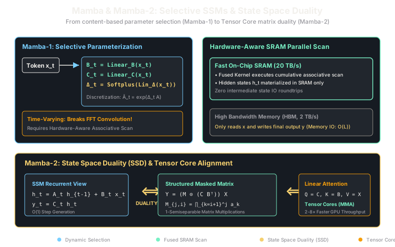
Mamba (Mamba-1) broke this trade-off by making the state space parameters dynamic functions of the current input token $x_t$. However, making parameters time-varying destroys the convolutional representation: the convolution kernel $\bar{K}$ can no longer be precomputed, rendering standard FFT parallelization impossible. Mamba resolved this with a hardware-aware parallel associative scan executed directly in fast GPU on-chip SRAM.

Mamba-2 pushed this paradigm further by proving State Space Duality (SSD): a theoretical equivalence showing that selective SSMs and masked linear attention are dual perspectives of the same 1-semiseparable matrix transformation. By reformulating the recurrence as structured block-matrix multiplications, Mamba-2 utilizes GPU Tensor Cores natively, achieving 2 to 8 times higher training throughput than Mamba-1.

Before analyzing selective mechanics, make sure you understand the foundational continuous formulation in state-space models and quadratic attention in transformers.

Think of It Like This

How It Actually Works

Selective State Spaces, SRAM Fusion, and State Space Duality

1. The Mamba-1 Selection Mechanism

In Mamba-1, input sequence $x \in \mathbb{R}^{B \times L \times D}$ passes through linear projection layers to dynamically generate time-varying discretization step sizes and projection matrices:

Here, $B_t \in \mathbb{R}^{B \times L \times N}$ and $C_t \in \mathbb{R}^{B \times L \times N}$ vary for each token, and $\Delta_t \in \mathbb{R}^{B \times L \times D}$ acts as a content-based gating mechanism. The continuous diagonal matrix $A \in \mathbb{R}^{D \times N}$ is discretized via zero-order hold (ZOH):

The recurrent update equation becomes:

When $\Delta_t \to 0$, $\bar{A}_t \to I$ and $\bar{B}_t \to 0$: the current input $x_t$ is ignored, and previous state $h_{t-1}$ is preserved indefinitely. When $\Delta_t$ is large, $\bar{A}_t \to 0$ and $\bar{B}_t$ absorbs $x_t$: the model resets its state and overwrites memory with fresh information.

2. Hardware-Aware Parallel Scan

Because $\bar{A}_t$ varies with time $t$, global convolution is mathematically invalid. A naive sequential loop over $L = 100{,}000$ steps on a GPU would cause severe memory bandwidth bottlenecks because reading and writing the state tensor $h \in \mathbb{R}^{B \times L \times D \times N}$ across High-Bandwidth Memory (HBM, ~2 TB/s) is catastrophically slow.

Mamba bypasses HBM by fusing the scan into a single GPU kernel:

1. Load parameters $(x, \Delta, A, B, C)$ from HBM to fast on-chip SRAM (~20 TB/s).
2. Discretize $\bar{A}_t, \bar{B}_t$ in SRAM.
3. Execute a parallel associative prefix scan (Blelloch scan) across time steps directly within GPU thread blocks.
4. Compute $y_t = C_t h_t$ and write only the final output $y \in \mathbb{R}^{B \times L \times D}$ back to HBM.

Intermediate states $h_t$ are never saved to global GPU memory during the forward pass; they are recomputed on the fly during backpropagation via kernel recomputation.

3. Mamba-2 and State Space Duality (SSD)

Mamba-2 constrains the transition matrix $A$ to be a scalar multiplier per channel ($A \in \mathbb{R}$, scaled by identity $I_N$). This simplifies the transformation into a 1-semiseparable matrix $M$:

The entire SSM operation over sequence length $L$ can be expressed as:

Comparing this to causal linear attention $Y = \left( \text{Mask} \circ (Q K^T) \right) V$, the mapping is exact:

• Query $Q = C$
• Key $K = B$
• Value $V = X$
• Attention Mask $M_{j, i}$ is weighted by cumulative decay factors $\prod a_k$.

Because $Y = (M \circ (C B^T)) X$ is a structured matrix multiplication, Mamba-2 partitions the sequence into blocks (e.g., block size 64) and executes the intra-block computations using GPU Tensor Cores (Matrix Multiply-Accumulate / MMA instructions). This bridges the hardware utilization gap between SSMs and Transformers.

Worked Example

Consider a single state dimension ($N = 1$) over 2 time steps ($t=1, 2$) showing how $\Delta_t$ selectively retains or forgets memories:

Parameters:

Time step 1 (Important token):

Let the model predict a large step size: $\Delta_1 = 2.0$.

Assuming initial state $h_0 = 0.0$:

Token $x_1$ is absorbed into the state vector.

Time step 2 (Irrelevant distractor token):

The model encounters filler content and selects a tiny step size: $\Delta_2 = 0.01$.

Updating the state:

Notice that even though distractor input $x_2$ had twice the magnitude of $x_1$ ($20.0$ vs $10.0$), the selective gate $\Delta_2$ suppressed $x_2$'s contribution to just $0.20$, while preserving 99% of prior memory $h_1$ ($19.80$).

Code

Here is a minimal, self-contained Python implementation of the selective associative scan showing how content-dependent $\Delta$ modulates state evolution:

1import numpy as np2
3
4def selective_ssm_step(5    x: np.ndarray, delta: np.ndarray, a_scalar: float, b: np.ndarray, c: np.ndarray6) -> np.ndarray:7    """Simulate a selective SSM forward pass across sequence length L."""8    seq_len = x.shape[0]9    state_dim = b.shape[1]10    y = np.zeros(seq_len)11
12    h = np.zeros(state_dim)13
14    for t in range(seq_len):15        # Discretize continuous parameters based on input-dependent delta[t]16        a_bar = np.exp(delta[t] * a_scalar)17        b_bar = delta[t] * b[t]18
19        # Selective recurrent state update20        h = a_bar * h + b_bar * x[t]21        y[t] = np.dot(c[t], h)22
23    return y24
25
26# Sequence of 3 tokens: Token 0 (signal), Token 1 (noise), Token 2 (query)27x = np.array([5.0, 100.0, 1.0])28# Model chooses high delta for important token, tiny delta for noise29delta = np.array([1.5, 0.001, 1.0])30
31a_scalar = -1.032b = np.array([[1.0], [1.0], [1.0]])  # State dimension N = 133c = np.array([[1.0], [1.0], [1.0]])34
35outputs = selective_ssm_step(x, delta, a_scalar, b, c)36
37print(f"Token inputs:    {x}")38print(f"Selective delta: {delta}")39print(f"Model outputs:   {np.round(outputs, 4)}")40# -> Token inputs:    [  5. 100.   1.]41# -> Selective delta: [1.5   0.001 1.   ]42# -> Model outputs:   [7.5    7.5925 3.7915]

Watch Out For

The Quick Version

• Mamba replaces static LTI state spaces with content-dependent parameters $B(x), C(x), \Delta(x)$.
• Content-dependent gating allows Mamba to selectively filter noise and retain critical facts across long horizons.
• Because selection breaks FFT convolution, Mamba uses a hardware-aware parallel scan executed entirely in fast GPU SRAM.
• Mamba-2 introduces State Space Duality (SSD), proving the mathematical equivalence of selective SSMs and masked linear attention.
• Mamba-2 executes intra-chunk recurrence using GPU Tensor Cores, achieving dramatic training throughput gains over Mamba-1.

What to Read Next

• Jamba: Hybrid SSM-Transformer
• Physics-Informed Scientific ML
• Backpropagation