Core ML

Double Descent

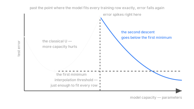
Push capacity past the point where a model fits every training row exactly and test error spikes, then falls again — often below the U-curve's first minimum.

Test error traces the classical U, spikes at the interpolation threshold where the model has just enough parameters to fit every training row, then descends a second time to below the first minimum

Why Does This Exist?

You're predicting the sugar content of grape batches from a near-infrared spectrum — 200 wavelength bands in, one number out — and you have 100 batches whose sugar was measured in a lab. The question is how big a model to fit.

The classical answer is a curve everyone can draw. Error against capacity is U-shaped: too few parameters and the model can't express the relationship, too many and it memorises. That's the bias-variance tradeoff, and its instruction is clear — find the bottom of the U, and never ship more parameters than data points.

Here's the wall. Past the bottom the error does climb, exactly as promised, all the way to a spike. Then it comes back down. Keep adding parameters and test error falls a second time, below the first minimum. Further down, 20 features score 1.188, the spike 3083, and 2,000 features 0.693 — half the error of the model the rule told you to ship. Not an artefact either: the same shape turns up in least squares, random features, forests and networks, characterised across all of them in 2019.

Think of It Like This

Bending a steel strip through a row of nails

Nails hammered into a board at various heights, and you want a strip of steel touching every head.

Take a short, stiff strip. It bridges over several nails and won't reach them: the left side of the U.

Now take a strip exactly long and flexible enough to reach all of them, no more. There's essentially one way to bend it, and the strip kinks hard between the nails, shooting off wildly where nothing constrains it. Every nail touched, the board described terribly. That's the spike.

Now take a strip five times longer. Countless ways to touch all the nails now, and among them long gentle curves that barely bend. Clamp on a spring pulling it toward straight, let go, and it settles into one of those.

More capacity didn't tighten the fit. It made room for a better shape among the tight fits, and something else had to choose.

How It Actually Works

The interpolation threshold

Add parameters and eventually the model fits every training row exactly — training error zero, or close enough that it stops moving. That's the interpolation threshold. For linear models with independent columns it's where parameter count equals row count: 100 random features against 100 batches.

Test error spikes there, not past it. The reason is the strip that was exactly long enough: at the threshold essentially one setting fits the data, so the fit takes whatever coefficients the equations force — and those are huge, because 100 constraints against 100 knobs leaves no slack.

Why the second descent happens

Push past the threshold and the constraint stops binding. With 2,000 features and 100 rows infinitely many settings fit the data exactly, so something other than the data picks one — and its preference happens to be good.

Gradient descent from small weights on a least-squares problem converges to the exact fit with the smallest coefficients:

\hat{w} \;=\; \arg\min_{w} \; \lVert w \rVert_2 \quad \text{subject to} \quad Xw = y

$X$ is the training features, $y$ the measured sugar contents, $w$ the coefficients, and $\lVert w \rVert_2$ their Euclidean length. Of all the perfect fits, take the one with the smallest coefficients — the smoothest one. Nobody asked for that; it's what gradient descent does when the answer is underdetermined.

So capacity and effective capacity come apart. Parameter count says how many knobs exist; effective capacity says how much the fit wiggles, and past the threshold the second falls while the first climbs. That gap is what the classical U assumed away.

What it cost

One clean rule left the table. Parameter count stopped being a usable proxy for the variance term, so "don't use more parameters than data points" is no longer actionable — the second descent lives entirely in the region that rule forbids. Model size is something you measure now, not derive.

What did not break is the bias-variance decomposition. It's exact algebra for squared loss and holds here unamended — the variance term really is enormous at the spike and really does shrink after. Only the mapping onto parameter count failed.

The shape shows up along other axes too, training time and sample size among them. And explicit regularisation flattens the spike: tuned weight decay or ridge makes the whole curve monotone.

Show Me the Code

Random features on the grape spectra, 100 batches, no regularisation.

1import numpy as np2
3
4def test_error(features: int, n: int = 100, trials: int = 8) -> float:5    rng, errs = np.random.default_rng(features), []6    for _ in range(trials):7        W = rng.normal(size=(200, features)) / np.sqrt(200)   # fixed random projection8        Xtr, Xte = rng.normal(size=(n, 200)), rng.normal(size=(2000, 200))9        b = rng.normal(size=200) / np.sqrt(200)10        ytr = Xtr @ b + rng.normal(0.0, 0.3, n)               # lab assay noise on sugar11        w = np.linalg.pinv(Xtr @ W) @ ytr                     # minimum-norm exact fit12        errs.append(np.mean((Xte @ W @ w - Xte @ b) ** 2))13    return float(np.mean(errs))14
15
16for p in (20, 60, 100, 140, 400, 2000):17    print(f"{p:5d} features   test MSE {test_error(p):7.3f}")18# ->    20 features   test MSE   1.18819# ->    60 features   test MSE   1.80620# ->   100 features   test MSE 3083.38221# ->   140 features   test MSE   2.43522# ->   400 features   test MSE   0.79523# ->  2000 features   test MSE   0.693

Twenty features is the classical sweet spot, sixty is worse on schedule, and at 100 — one feature per batch — the model interpolates and test error is 2,600 times the sweet spot's. By 2,000 the error is 0.693, under the 1.188 the U-curve pointed at. pinv does the work: below the threshold it's ordinary least squares, above it, the smallest-coefficient exact fit.

Watch Out For

Reading it as permission to skip regularisation

The story is seductive: overparameterise hard enough and the geometry regularises for you, so weight decay is a relic. Then the training bill arrives — the far end of that curve took twenty times the parameters of the first minimum, for a factor of two.

Tuned ridge or weight decay usually removes the spike and lands at the same error or better, for a fraction of the compute. A monotone curve also makes model size a boring decision rather than a hazard. It's the cheaper lever almost every time.

Expecting to see it on a tuned tree ensemble over 5,000 tabular rows

You sweep the number of trees, or the depth, looking for a spike. Test error gets slightly worse then plateaus, so you conclude the effect is overstated.

It belongs to the interpolating regime, and a depth-limited, early-stopped ensemble never enters it. Check training error first: if it isn't collapsing to essentially zero somewhere in your sweep, there's no interpolation threshold on your plot and no spike to find. Reproducing it means removing the guardrails — unlimited depth, no shrinkage, no early stopping — the honest reason it rarely changes a tabular workflow.

The Quick Version

The classical U says test error rises once capacity passes the sweet spot. Past the interpolation threshold — just enough capacity to fit every training row exactly — it spikes, then descends a second time, often below the first minimum.
At the threshold one exact fit exists and it needs enormous coefficients. Past it there are many, and gradient descent's preference for small coefficients picks a smooth one.
Capacity and effective capacity come apart, so model size is something you measure. The bias-variance identity is untouched — only the mapping onto parameter count broke.
Tuned weight decay or ridge flattens the spike, usually cheaper than overparameterising past it.