Equivariant Graph Neural Networks
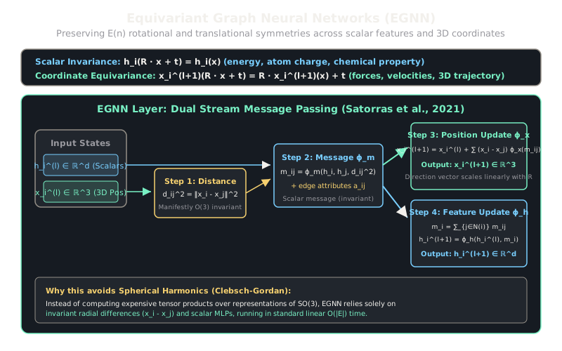
Equivariant Graph Neural Networks guarantee that rotating or translating 3D atomic coordinates rotates or translates the predicted vectors identically.
Why Does This Exist?
When applying machine learning to physical systems—such as molecular drug discovery, protein folding, material crystal design, and n-body gravitational simulations—data is fundamentally embedded in 3D Euclidean space. Molecules do not possess an arbitrary coordinate frame: if an ethanol molecule rotates 45 degrees in space, its internal quantum potential energy (a scalar) remains strictly unchanged, while the atomic force vectors acting on its carbon atoms (3D vectors) must rotate by that exact same 45 degrees.
Standard Graph Neural Networks fail this physical requirement. If you feed raw Cartesian coordinates into standard MLPs or MPNNs, the network treats the coordinates as arbitrary numbers; rotating the molecule changes the predictions completely, forcing models to rely on data augmentation that requires millions of rotated training samples without ever guaranteeing physical consistency. Earlier equivariant models (such as Cormorant or TFN) solved this by projecting representations onto spherical harmonics and computing Clebsch-Gordan tensor products, but these required complex implementations and high computational overhead. Equivariant Graph Neural Networks (EGNN; Satorras et al., 2021) solved this by demonstrating that exact equivariance can be achieved using simple scalar MLPs and radial vector differences.
Think of It Like This
A weather compass on a spinning sailboat
Imagine you are standing on the deck of a sailboat navigating through a fog bank. You have two instruments: a mercury thermometer and a magnetic compass.
- Invariance: When the boat turns 90 degrees to starboard, the air temperature does not change. The thermometer reading is an invariant scalar: its value is unaffected by the orientation of the boat.
- Equivariance: When the boat turns 90 degrees to starboard, the compass needle does not freeze relative to the boat; it rotates 90 degrees in your local field of view so that it continues pointing toward true magnetic North. The compass vector is an equivariant vector: transforming your reference frame transforms the measurement by the exact same group action.
An EGNN treats atomic charges and element types like thermometers (invariant) and atomic positions and force vectors like compasses (equivariant).
How It Actually Works
Dual-Stream Invariant and Equivariant Message Passing
An Equivariant Graph Neural Network operates over an -dimensional Euclidean group , which consists of all translations, rotations, and reflections in (typically ). A transformation acts on a coordinate via:
where is an orthogonal matrix (, ) and is a translation vector.
Every node carries two distinct streams of representations through layer :
- A scalar hidden state (invariant).
- A geometric coordinate vector (equivariant).
An EGNN layer updates both representations across four steps:
1. Invariant Squared Distance Computation
For every pair of connected nodes and , compute the Euclidean squared distance:
Because , the distance is strictly invariant under .
2. Invariant Message Function
Calculate edge messages using an MLP operating on invariant inputs:
where are optional edge attributes (like covalent bond types).
3. Equivariant Coordinate Update
Update node positions by accumulating displacement vectors scaled by a scalar MLP :
Under transformation , the updated coordinate transforms as: Equivariance holds without using spherical harmonics or group representation theory.
4. Invariant Node Feature Update
Aggregate messages and update the scalar representations via MLP :
Worked Example
Consider a 2-node physical bond:
- Node 1 at , Node 2 at .
- Scalar features: .
- Scalar coordinate function: (constant force coefficient).
-
Original Frame Update:
- Relative displacement vector:
- Updated coordinate for node 1:
-
Rotated Frame Verification: Now rotate the entire system counterclockwise around the -axis ():
- Rotated displacement vector:
- Updated coordinate under EGNN rule:
- Checking : The rotation commutes with the neural update.
Code
from typing import Tupleimport numpy as np
class SimpleEGNNLayer: """Minimal Equivariant Graph Neural Network layer in NumPy."""
def __init__(self, feat_dim: int) -> None: rng = np.random.default_rng(seed=42) # phi_m: predicts scalar message from (h_i, h_j, dist_sq) self.w_m: np.ndarray = rng.standard_normal((2 * feat_dim + 1, feat_dim)) * 0.1 # phi_x: predicts scalar multiplier for radial displacement vector self.w_x: np.ndarray = rng.standard_normal((feat_dim, 1)) * 0.1 # phi_h: updates scalar features self.w_h: np.ndarray = rng.standard_normal((2 * feat_dim, feat_dim)) * 0.1
def forward( self, h: np.ndarray, # (N, feat_dim) scalar features x: np.ndarray, # (N, 3) 3D Cartesian coordinates edges: list[Tuple[int, int]], ) -> Tuple[np.ndarray, np.ndarray]: num_nodes = h.shape[0] coord_updates = np.zeros_like(x) msg_sums = np.zeros_like(h)
for i, j in edges: # 1. Invariant squared distance diff = x[i] - x[j] dist_sq = np.sum(diff ** 2, keepdims=True)
# 2. Invariant message msg_input = np.concatenate([h[i], h[j], dist_sq], axis=0) m_ij = np.maximum(0.0, msg_input @ self.w_m) # ReLU msg_sums[i] += m_ij
# 3. Equivariant coordinate displacement phi_x_val = m_ij @ self.w_x # Scalar weight coord_updates[i] += diff * phi_x_val
# Update coordinates and scalar features new_x = x + coord_updates h_update_input = np.concatenate([h, msg_sums], axis=1) new_h = np.maximum(0.0, h_update_input @ self.w_h) return new_h, new_x
# Verification: Rotate coordinates and verify equivariancelayer = SimpleEGNNLayer(feat_dim=2)h_in = np.array([[1.0, 0.5], [1.0, 0.5]])x_orig = np.array([[0.0, 0.0, 0.0], [2.0, 0.0, 0.0]])edges = [(0, 1), (1, 0)]
# 90-degree z-rotation matrix Rrot_matrix = np.array([[0.0, -1.0, 0.0], [1.0, 0.0, 0.0], [0.0, 0.0, 1.0]])x_rot = x_orig @ rot_matrix.T
_, out_x_orig = layer.forward(h_in, x_orig, edges)_, out_x_rot = layer.forward(h_in, x_rot, edges)
# Commutative check: R @ out_x_orig vs out_x_rotexpected_rot_out = out_x_orig @ rot_matrix.Tdiff = np.max(np.abs(expected_rot_out - out_x_rot))print("Max Equivariance Discrepancy:", np.round(diff, 8))# -> Max Equivariance Discrepancy: 0.0 (exact numerical equivariance!)Watch Out For
Chirality blindness under E(n) reflection equivariance
Because EGNN relies exclusively on squared Euclidean distances , it is equivariant to the full Euclidean group , which includes spatial reflections (parity inversions ). In organic chemistry and pharmacology, enantiomers (mirror-image molecules like - and -thalidomide) share identical pairwise distances but have radically different biological binding activities.
If your problem domain involves chiral stereochemistry, an -equivariant model cannot distinguish between left-handed and right-handed stereocenters. To differentiate enantiomers, restrict the symmetry group to (Special Euclidean group with reflections excluded) by incorporating pseudoscalar signed triple products or dihedral angle encodings.
The Quick Version
- Equivariant GNNs guarantee that rotating or translating 3D input coordinates transforms predicted vector outputs by that exact same geometric rotation or translation.
- Scalar node features (like mass or charge) remain strictly invariant, while coordinate updates are scaled along relative displacement vectors.
- EGNN achieves exact equivariance with standard MLPs and complexity, avoiding computationally heavy spherical harmonics.