Graph Transformers

Graph Transformers replace local message passing with full pairwise attention augmented by shortest-path distances and node centrality encodings.

Graphormer injects degree centrality encodings into input tokens and biases all-to-all attention logits with shortest-path topological distances and edge features

Why Does This Exist?

For years, the standard inductive bias for graph neural networks was strict spatial locality: nodes were only allowed to pass messages directly to their immediate 1-hop neighbors along existing graph edges. However, in many critical graph domains—such as molecular chemistry, where atoms on opposite sides of a folded protein interact through non-covalent electromagnetic fields—forcing information to crawl hop-by-hop along a sparse chain of edges creates severe over-squashing and gradient vanishing bottlenecks.

Standard NLP Transformers (like BERT and GPT) compute dense, all-to-all self-attention, allowing every token to communicate directly with every other token in a single layer. But naively treating a graph as an unordered set of tokens fed into a vanilla Transformer completely destroys graph topology: the model has no way of knowing whether two nodes are separated by 1 bond or 20 bonds. Graph Transformers—epitomized by Graphormer (Ying et al., NeurIPS 2021)—solved this dilemma by marrying the unconstrained expressive capacity of global self-attention with mathematical inductive biases that encode graph centrality, shortest-path spatial distances, and edge attributes directly into the attention matrix.

Think of It Like This

A United Nations summit with simultaneous translators

Imagine a summit with delegates from 50 nations seated in a giant conference hall.

Classical MPNN: Delegates can only whisper to the two delegates seated immediately to their left and right. If the delegate from Japan wants to coordinate a climate treaty with the delegate from Chile, their proposal must be whispered through 25 intermediate delegates. By the time it arrives, the proposal is mangled and distorted.
Vanilla Transformer: All delegates wear headsets that broadcast everyone's voice equally into one chaotic auditory room. Nobody knows who shares a land border, who shares an ocean, or who sits in the same trade bloc.
Graph Transformer (Graphormer): Every delegate can speak directly to any other delegate across the room in one second (global attention). But the translator's earpiece automatically applies an auditory distance volume filter: proposals from immediate border neighbors come through loudest, while proposals from across the globe arrive with clear geographic distance labels.

How It Actually Works

The Graphormer Architectural Blueprint

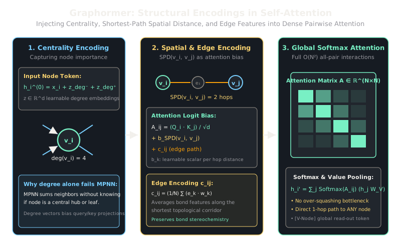
Graphormer treats a graph of $N$ nodes as a sequence of $N$ tokens, allowing full $\mathcal{O}(N^2)$ pairwise attention while encoding topological structure through three explicit architectural mechanisms:

1. Centrality Encoding

Standard Transformers lack awareness of node degree or topological centrality. Graphormer assigns two learnable embedding vectors $\mathbf{z}_{\deg^-(v_i)}^-, \mathbf{z}_{\deg^+(v_i)}^+ \in \mathbb{R}^d$ based on the indegree and outdegree of node $v_i$ . The initial input representation $\mathbf{h}_i^{(0)}$ combines the raw feature vector $\mathbf{x}_i$ with these degree embeddings:

$\mathbf{h}_i^{(0)} = \mathbf{x}_i + \mathbf{z}_{\deg^-(v_i)}^- + \mathbf{z}_{\deg^+(v_i)}^+$

This allows the attention queries and keys to naturally modulate attention strength based on whether a node is a high-degree hub or a peripheral leaf.

2. Spatial Encoding via Shortest-Path Distance (SPD)

To preserve graph connectivity without restricting attention to adjacent edges, Graphormer computes the shortest-path distance $\phi(v_i, v_j)$ between every node pair $(v_i, v_j)$ (setting $\phi = -1$ if nodes belong to disconnected components).

A learnable scalar bias $b_{\phi(v_i, v_j)} \in \mathbb{R}$ is added directly to the self-attention logit:

$A_{ij} = \frac{(\mathbf{h}_i \mathbf{W}_Q)(\mathbf{h}_j \mathbf{W}_K)^\top}{\sqrt{d}} + b_{\phi(v_i, v_j)}$

If $v_i$ and $v_j$ are immediate 1-hop neighbors ( $\phi = 1$ ), the model learns a strong positive bias $b_1$ ; if they are 10 hops apart, $b_{10}$ attenuates the attention score while still permitting direct gradient flow.

3. Edge Feature Encoding

In molecules, edges carry critical physical information (single vs. double bonds, aromatic rings, conjugated systems). For a node pair $(v_i, v_j)$ , let $\mathcal{P}_{ij} = (e_1, e_2, \dots, e_K)$ be the sequence of edges along the shortest path between them. Graphormer projects the edge features $\mathbf{x}_{e_k}$ using learnable weights $\mathbf{w}_k^E$ and averages them into an edge bias $c_{ij}$ :

$c_{ij} = \frac{1}{K} \sum_{k=1}^K \mathbf{x}_{e_k}^\top \mathbf{w}_k^E$

The final attention logit is:

$\hat{A}_{ij} = \frac{(\mathbf{h}_i \mathbf{W}_Q)(\mathbf{h}_j \mathbf{W}_K)^\top}{\sqrt{d}} + b_{\phi(v_i, v_j)} + c_{ij}$

The updated representations are obtained via standard multi-head softmax:

$\mathbf{h}_i^{(l+1)} = \sum_{j=1}^N \text{Softmax}\left(\hat{A}_{ij}\right) \left(\mathbf{h}_j^{(l)} \mathbf{W}_V\right)$

Worked Example

Consider nodes $i$ and $j$ in a molecular graph. Let hidden dimension $d = 4$ :

Query projection $\mathbf{q}_i = [1.0, 0.0, 1.0, 0.0]^\top$ .
Key projection $\mathbf{k}_j = [0.0, 1.0, 1.0, 0.0]^\top$ .
$\sqrt{d} = \sqrt{4} = 2.0$ .
Shortest-path distance between $i$ and $j$ is $\phi(v_i, v_j) = 1$ (immediate neighbors). Learned spatial bias $b_1 = 1.5$ .
Path contains 1 double bond with encoded edge bias $c_{ij} = 0.5$ .

Dot-Product Attention Score: $\mathbf{q}_i^\top \mathbf{k}_j = (1 \times 0) + (0 \times 1) + (1 \times 1) + (0 \times 0) = 1.0$ $\text{Scaled dot-product} = \frac{1.0}{2.0} = 0.5$
Add Spatial and Edge Encodings: $\hat{A}_{ij} = 0.5 + b_1 + c_{ij} = 0.5 + 1.5 + 0.5 = 2.5$

Compare this against node $k$ which has identical dot-product $\mathbf{q}_i^\top \mathbf{k}_k / 2 = 0.5$ but sits 4 hops away ( $\phi = 4, b_4 = -2.0, c_{ik} = 0.0$ ): $\hat{A}_{ik} = 0.5 + (-2.0) + 0.0 = -1.5$

Softmax Comparison: The unnormalized attention weights are $e^{2.5} \approx 12.18$ versus $e^{-1.5} \approx 0.22$ . The spatial bias ensures the local bond receives $\approx 55\times$ more attention weight than the 4-hop neighbor, while still leaving the long-range path open for critical multi-hop signals.

Code

1import numpy as np2
3
4def graphormer_attention(5    node_features: np.ndarray,      # Shape: (N, d)6    shortest_path_dist: np.ndarray, # Shape: (N, N) matrix of hop distances7    w_q: np.ndarray,                # Shape: (d, d)8    w_k: np.ndarray,                # Shape: (d, d)9    w_v: np.ndarray,                # Shape: (d, d)10    spatial_biases: np.ndarray,     # Shape: (max_dist + 1,) learnable scalar biases11) -> np.ndarray:12    """Single-head Graphormer attention layer with shortest-path spatial bias."""13    num_nodes, d = node_features.shape14
15    # 1. Linear Query, Key, Value projections16    q = node_features @ w_q  # (N, d)17    k = node_features @ w_k  # (N, d)18    v = node_features @ w_v  # (N, d)19
20    # 2. Scaled dot-product attention logits: (N, N)21    logits = (q @ k.T) / np.sqrt(d)22
23    # 3. Add shortest-path distance spatial bias24    spatial_matrix = spatial_biases[shortest_path_dist]25    augmented_logits = logits + spatial_matrix26
27    # 4. Softmax over all j28    exp_logits = np.exp(augmented_logits - np.max(augmented_logits, axis=-1, keepdims=True))29    attn_weights = exp_logits / np.sum(exp_logits, axis=-1, keepdims=True)30
31    # 5. Output pooling32    out = attn_weights @ v33    return out34
35
36# Test with 3-node path: 0 - 1 - 237spd = np.array([38    [0, 1, 2],39    [1, 0, 1],40    [2, 1, 0],41], dtype=np.int32)42
43feat = np.array([44    [1.0, 0.0],45    [0.0, 1.0],46    [1.0, 1.0],47])48
49# Spatial biases: b_0=0.0, b_1=2.0 (boost 1-hop), b_2=-1.0 (attenuate 2-hop)50biases = np.array([0.0, 2.0, -1.0])51w = np.eye(2)52
53output_embeddings = graphormer_attention(feat, spd, w, w, w, biases)54print("Graphormer output representations shape:", output_embeddings.shape)55# -> Graphormer output representations shape: (3, 2)56print("Node 0 updated embedding:", np.round(output_embeddings[0], 4))

Watch Out For

The quadratic O(N^2) memory barrier on large graphs

Because Graphormer computes pairwise self-attention between every pair of nodes, its computational and memory complexity scales as $\mathcal{O}(N^2)$ in the number of nodes. While this is acceptable for small-to-medium graphs like molecules and proteins ( $N < 500$ ), applying full Graphormer to social networks, citation graphs, or transaction systems ( $N > 100{,}000$ ) causes immediate GPU Out-Of-Memory errors.

On large-scale graphs, do not compute full dense self-attention across the whole node set. Use sparse graph transformer variants—such as NodeFormer, Exphormer, or Performer/Kernelized linear attention—or apply sub-graph sampling (like Ego-graph tokenization) to bound the sequence length $N$ .

The Quick Version

Graph Transformers overcome the locality bottleneck of MPNNs by enabling global pairwise self-attention across all node pairs.
Graphormer injects graph inductive biases using degree centrality encodings and shortest-path distance spatial bias terms.
Edge features along shortest paths are averaged directly into attention logits, capturing chemical bond structures across arbitrary topological distances.