Spectral Graph Convolutions

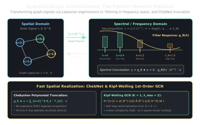
Spectral graph convolutions define filtering on networks by transforming signals into the Graph Laplacian's frequency domain using its eigenvectors.

Spectral graph convolution projects spatial node signals onto Laplacian eigenvectors, multiplies by frequency filter coefficients, and reconstructs via inverse Fourier transform

Why Does This Exist?

In classical image processing, convolution is defined through sliding filters: because pixels sit on a uniform, translation-invariant grid, shifting a $3 \times 3$ kernel one pixel to the right preserves its spatial meaning everywhere on the image. On a graph, sliding a filter spatially is ill-defined: node degrees vary arbitrarily, there is no canonical "left" or "right", and reordering node indices produces arbitrary permutations.

By the convolution theorem of signal processing, convolution in the spatial domain corresponds to simple pointwise multiplication in the frequency domain. Spectral Graph Theory generalizes this principle to arbitrary graphs by using the eigenvectors of the Graph Laplacian as the Fourier basis. Spectral graph convolutions established the mathematical foundation of modern geometric deep learning, explaining why graph convolutions behave as low-pass filters and providing the mathematical derivation that yielded the ubiquitously used Graph Convolutional Network (GCN).

Think of It Like This

Equalizing an audio track with a sound mixer

Imagine an acoustic recording containing an orchestra. In the raw time domain (sound wave pressure over seconds), bass notes, violins, and cymbals are tangled together in a single oscillating waveform. If you want to boost the cello and quiet the flute, operating directly on time samples is agonizingly difficult.

Instead, a sound engineer runs a Fourier transform. This breaks the single tangled wave into an equalizer spectrum: bass notes occupy low frequencies (slow vibrations), while flutes and cymbals occupy high frequencies (rapid vibrations). The engineer adjusts specific frequency slider knobs ( $g_\theta(\lambda)$ ) and then runs an inverse Fourier transform back to audio.

Spectral graph convolution does the exact same thing to graph signals: smooth, community-level trends correspond to low Laplacian frequencies, while sharp node-to-node discrepancies correspond to high frequencies.

How It Actually Works

The Graph Fourier Transform and ChebNet Derivation

Given an undirected graph $G = (V, E)$ with adjacency matrix $\mathbf{A} \in \{0, 1\}^{N \times N}$ and degree matrix $\mathbf{D}_{ii} = \sum_j A_{ij}$ , the unnormalized Graph Laplacian is $\mathbf{L} = \mathbf{D} - \mathbf{A}$ . The symmetric normalized Laplacian is:

$\mathbf{L}_{\text{sym}} = \mathbf{I}_N - \mathbf{D}^{-1/2} \mathbf{A} \mathbf{D}^{-1/2}$

Because $\mathbf{L}_{\text{sym}}$ is real, symmetric, and positive semi-definite, it admits an eigendecomposition $\mathbf{L}_{\text{sym}} = \mathbf{U} \mathbf{\Lambda} \mathbf{U}^\top$ , where:

$\mathbf{U} = [\mathbf{u}_1, \dots, \mathbf{u}_N] \in \mathbb{R}^{N \times N}$ is the orthonormal matrix of eigenvectors (the graph Fourier basis).
$\mathbf{\Lambda} = \text{diag}(\lambda_1, \dots, \lambda_N)$ with eigenvalues $0 = \lambda_1 \le \lambda_2 \le \dots \le \lambda_N \le 2$ acting as the graph frequencies.

1. Forward and Inverse Graph Fourier Transform

For a spatial node signal $\mathbf{x} \in \mathbb{R}^N$ , the Graph Fourier Transform $\hat{\mathbf{x}}$ and its inverse are:

$\hat{\mathbf{x}} = \mathbf{U}^\top \mathbf{x}, \qquad \mathbf{x} = \mathbf{U} \hat{\mathbf{x}}$

2. Spectral Filtering

Convolving a signal $\mathbf{x}$ with a parameterized filter $g_\theta$ in the spectral domain is defined as:

$\mathbf{y} = g_\theta \star \mathbf{x} = \mathbf{U} g_\theta(\mathbf{\Lambda}) \mathbf{U}^\top \mathbf{x}$

where $g_\theta(\mathbf{\Lambda}) = \text{diag}(\theta_1, \dots, \theta_N)$ is a diagonal matrix of learnable spectral filter multipliers.

3. ChebNet Truncation

Evaluating $\mathbf{U} g_\theta(\mathbf{\Lambda}) \mathbf{U}^\top$ requires computing the full eigendecomposition of $\mathbf{L}$ , which costs $\mathcal{O}(N^3)$ and does not yield spatially localized filters. Defferrard et al. (2016) resolved this by approximating $g_\theta(\mathbf{\Lambda})$ with a truncated expansion of Chebyshev polynomials $T_k(x)$ up to order $K$ :

$g_\theta \star \mathbf{x} \approx \sum_{k=0}^K \theta_k T_k(\mathbf{\tilde{L}}) \mathbf{x}$

where $\mathbf{\tilde{L}} = \frac{2}{\lambda_{\max}} \mathbf{L}_{\text{sym}} - \mathbf{I}_N$ scales eigenvalues into $[-1, 1]$ , and polynomials satisfy recurrence $T_0(x) = 1$ , $T_1(x) = x$ , and $T_k(x) = 2x T_{k-1}(x) - T_{k-2}(x)$ . This formulation is strictly $K$ -hop spatially localized and costs only $\mathcal{O}(K |E|)$ .

4. The Kipf-Welling 1st-Order GCN Approximation

Kipf & Welling (2017) truncated ChebNet to $K = 1$ , assumed $\lambda_{\max} \approx 2$ , and set $\theta = \theta_0 = -\theta_1$ . Applying the "renormalization trick" $\mathbf{\tilde{A}} = \mathbf{A} + \mathbf{I}_N$ and $\mathbf{\tilde{D}}_{ii} = \sum_j \tilde{A}_{ij}$ collapses spectral convolution directly into the spatial GCN update rule:

$\mathbf{H}^{(l+1)} = \sigma\left( \mathbf{\tilde{D}}^{-1/2} \mathbf{\tilde{A}} \mathbf{\tilde{D}}^{-1/2} \mathbf{H}^{(l)} \mathbf{W}^{(l)} \right)$

Worked Example

Consider a 2-node graph connected by an edge ( $N = 2, A_{12} = A_{21} = 1$ ).

Adjacency $\mathbf{A} = \begin{bmatrix} 0 & 1 \\ 1 & 0 \end{bmatrix}$ , Degree $\mathbf{D} = \begin{bmatrix} 1 & 0 \\ 0 & 1 \end{bmatrix}$ .
Normalized Laplacian: $\mathbf{L}_{\text{sym}} = \mathbf{I} - \mathbf{D}^{-1/2}\mathbf{A}\mathbf{D}^{-1/2} = \begin{bmatrix} 1 & -1 \\ -1 & 1 \end{bmatrix}$
Eigendecomposition: $\lambda_1 = 0 \quad (\text{constant mode}), \quad \mathbf{u}_1 = \frac{1}{\sqrt{2}} \begin{bmatrix} 1 \\ 1 \end{bmatrix}$ $\lambda_2 = 2 \quad (\text{oscillating mode}), \quad \mathbf{u}_2 = \frac{1}{\sqrt{2}} \begin{bmatrix} 1 \\ -1 \end{bmatrix}$ $\mathbf{U} = \frac{1}{\sqrt{2}} \begin{bmatrix} 1 & 1 \\ 1 & -1 \end{bmatrix}$

Let the input signal be $\mathbf{x} = \begin{bmatrix} 4.0 \\ 2.0 \end{bmatrix}$ .

Compute Graph Fourier Transform $\hat{\mathbf{x}} = \mathbf{U}^\top \mathbf{x}$ : $\hat{x}_1 = \frac{1}{\sqrt{2}}(4.0 + 2.0) = \frac{6.0}{\sqrt{2}} \approx 4.2426 \quad (\text{low frequency energy})$ $\hat{x}_2 = \frac{1}{\sqrt{2}}(4.0 - 2.0) = \frac{2.0}{\sqrt{2}} \approx 1.4142 \quad (\text{high frequency energy})$
Apply Low-Pass Filter: Let filter coefficients be $\theta_1 = 1.0$ (preserve low frequency) and $\theta_2 = 0.0$ (cut high frequency): $\hat{\mathbf{y}} = g_\theta(\mathbf{\Lambda}) \hat{\mathbf{x}} = \begin{bmatrix} 1.0 \times \frac{6}{\sqrt{2}} \\ 0.0 \times \frac{2}{\sqrt{2}} \end{bmatrix} = \begin{bmatrix} \frac{6}{\sqrt{2}} \\ 0 \end{bmatrix}$
Inverse Fourier Transform $\mathbf{y} = \mathbf{U} \hat{\mathbf{y}}$ : $\mathbf{y} = \frac{1}{\sqrt{2}} \begin{bmatrix} 1 & 1 \\ 1 & -1 \end{bmatrix} \begin{bmatrix} \frac{6}{\sqrt{2}} \\ 0 \end{bmatrix} = \begin{bmatrix} 3.0 \\ 3.0 \end{bmatrix}$ The high-frequency discrepancy between node 1 (4.0) and node 2 (2.0) was smoothed out into the mean consensus (3.0, 3.0).

Code

1import numpy as np2
3
4def spectral_graph_convolution(5    signal: np.ndarray,       # Shape: (N,)6    adjacency: np.ndarray,    # Shape: (N, N)7    filter_weights: np.ndarray,  # Shape: (N,) learnable spectral multipliers8) -> np.ndarray:9    """Exact spectral graph convolution via Laplacian eigendecomposition."""10    num_nodes = signal.shape[0]11    degrees = np.sum(adjacency, axis=1)12
13    # Compute normalized Laplacian L_sym = I - D^(-1/2) * A * D^(-1/2)14    deg_inv_sqrt = 1.0 / np.sqrt(np.maximum(degrees, 1e-8))15    d_mat = np.diag(deg_inv_sqrt)16    l_sym = np.eye(num_nodes) - d_mat @ adjacency @ d_mat17
18    # Eigendecomposition: L_sym = U * Lambda * U.T19    eigenvalues, u_basis = np.linalg.eigh(l_sym)20
21    # 1. Forward Graph Fourier Transform22    x_hat = u_basis.T @ signal23
24    # 2. Spectral Filtering (pointwise multiplication in frequency domain)25    y_hat = filter_weights * x_hat26
27    # 3. Inverse Graph Fourier Transform28    y_spatial = u_basis @ y_hat29    return y_spatial30
31
32# Test with 2-node graph: 0 - 133a = np.array([[0.0, 1.0], [1.0, 0.0]])34x = np.array([4.0, 2.0])35# Low-pass filter: keep DC mode (index 0), suppress high frequency (index 1)36filter_w = np.array([1.0, 0.0])37
38smoothed_signal = spectral_graph_convolution(x, a, filter_w)39print("Smoothed signal:", np.round(smoothed_signal, 4))40# -> Smoothed signal: [3. 3.]

Watch Out For

Spectral domain domain-transfer failure

Spectral filters $g_\theta(\mathbf{\Lambda})$ are parameterized directly against the specific eigenvalues $\mathbf{\Lambda}$ and eigenvectors $\mathbf{U}$ of a fixed graph Laplacian $\mathbf{L}$ . Because the eigenvectors $\mathbf{U}$ depend fundamentally on the precise size and connectivity of that single graph, an exact spectral model cannot be transferred to a new, different graph topology.

If your dataset contains multiple graphs of varying sizes (such as molecular benchmarks like TU-MUTAG or ZINC), do not parameterize filters as raw eigenvector multipliers. Use polynomial spatial approximations (such as ChebNet or spatial GCN / MPNN) that operate via localized adjacency matrix multiplications and generalize across arbitrary graph domains.

The Quick Version

The Graph Fourier Transform uses the eigenvectors of the normalized Graph Laplacian as the orthogonal frequency basis.
Spectral convolution projects spatial node signals into the frequency domain, multiplies by filter multipliers, and performs an inverse transform.
ChebNet avoids expensive $\mathcal{O}(N^3)$ eigendecomposition by approximating spectral filters with truncated Chebyshev polynomials, deriving the spatial GCN.