Deep Time Series Architectures

Deep learning for time series replaces manual statistical modeling with neural building blocks designed specifically for temporal patterns. From interpretable backward-and-forward forecast stacks to causal dilated convolutions and patch-based transformers, these architectures capture complex multi-horizon dependencies.

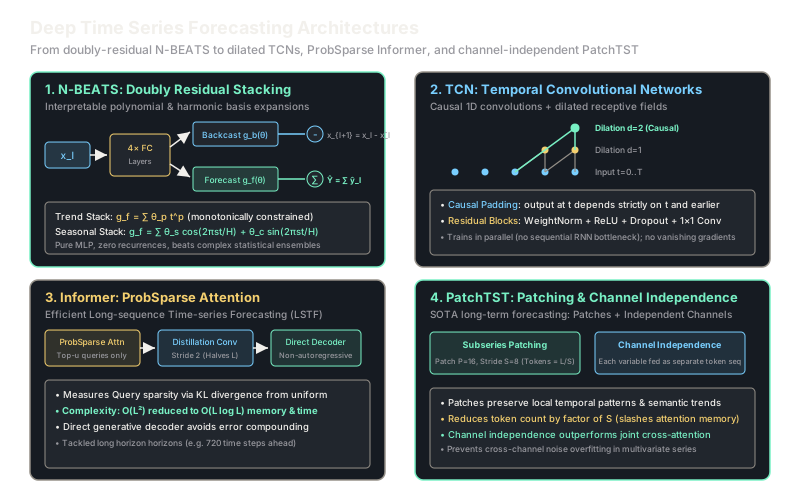
Four key deep forecasting architectures: N-BEATS doubly residual blocks, dilated causal TCNs, Informer ProbSparse attention, and PatchTST channel independence

Why Does This Exist?

Classical statistical forecasting methods like ARIMA, exponential smoothing (ETS), and vector autoregression (VAR) perform well on clean univariate series with short horizons. However, they struggle when scaling across thousands of interrelated series, long lookback windows ( $L > 500$ ), non-linear dynamics, or multi-horizon forecasts ( $H \ge 96$ ).

Early deep learning attempts simply applied standard recurrent networks (LSTMs and GRUs) to temporal sequences. But RNNs suffer from sequential compute bottlenecks, vanishing gradients over long horizons, and error compounding during iterative autoregressive rollouts.

To overcome these barriers, four landmark deep forecasting architectures emerged:

N-BEATS (2019): Demonstrated that a pure multi-layer perceptron (MLP) with doubly residual connections can beat statistical ensembles on the M4 competition without recurrence or attention.
Temporal Convolutional Networks (TCN, 2018): Replaced recurrent units with 1D causal dilated convolutions, achieving massive receptive fields and parallel training.
Informer (2021): Solved long sequence time-series forecasting (LSTF) by replacing quadratic $\mathcal{O}(L^2)$ attention with $\mathcal{O}(L \log L)$ ProbSparse attention.
PatchTST (2023): Revolutionized Transformer-based forecasting through subseries patching and channel independence, establishing state-of-the-art accuracy while slashing memory footprint.

Think of It Like This

Four ways to predict the weather for the next month

Imagine an atmospheric research bureau testing four different predictive strategies:

N-BEATS is the mathematical decomposition committee: It looks at historical barometric pressure, uses a dedicated desk to subtract the smooth multi-year warming trend, passes the remainder to another desk to subtract the repeating seasonal solstice wave, and sums their forward predictions.
TCN is the telescope array: Instead of inspecting every second sequentially, it uses lenses spaced exponentially further apart ( $1\text{ hour}, 2\text{ hours}, 4\text{ hours}, 8\text{ hours}$ ) to see months into the past in parallel without losing temporal order.
Informer is the executive summarizer: Rather than comparing every hour of last year with every other hour, it scans for anomalous storms, attends only to the most informative active weather queries, and predicts the entire month in one stroke.
PatchTST is the subseries jigsaw specialist: Instead of treating single hourly numbers as tokens, it groups consecutive days into compact semantic patches and forecasts temperature, wind, and pressure through independent channels to keep sensor noise from bleeding across variables.

How It Actually Works

Architectural Mechanics and Formulations

1. N-BEATS: Doubly Residual Basis Expansions

N-BEATS operates as a cascade of blocks organized into stacks. Each block $l$ receives historical input $x_l \in \mathbb{R}^L$ (where $x_1 = x$ is the original lookback window). The block consists of a 4-layer fully connected stack followed by two linear projection heads generating coefficient vectors $\theta_l^b$ (backcast) and $\theta_l^f$ (forecast):

\theta_l^b = \mathbf{W}_l^b h_{l,4}, \quad \theta_l^f = \mathbf{W}_l^f h_{l,4}

These coefficients parameterize basis functions $g_l^b$ and $g_l^f$ :

Backcast Output: $\hat{x}_l = g_l^b(\theta_l^b) \in \mathbb{R}^L$ reconstructs the historical input.
Forecast Output: $\hat{y}_l = g_l^f(\theta_l^f) \in \mathbb{R}^H$ predicts the future horizon.

The block applies a double residual update:

The backcast is subtracted from the block input to remove the signal it explained: $x_{l+1} = x_l - \hat{x}_l$
The final forecast is the sum of all individual block forecasts across all stacks: $\hat{Y} = \sum_{l=1}^B \hat{y}_l$

In interpretable N-BEATS, basis functions are constrained:

Trend Basis: Monomial powers of time $g_l^f(\theta_l^f) = \sum_{p=0}^P \theta_{l,p}^f t^p$ (linear, quadratic trends).
Seasonality Basis: Periodic Fourier harmonics $g_l^f(\theta_l^f) = \sum_{s=0}^S \left( \theta_{l,s}^f \cos\left(\frac{2\pi s t}{H}\right) + \theta_{l,s+S}^f \sin\left(\frac{2\pi s t}{H}\right) \right)$ .

2. Temporal Convolutional Networks (TCN)

A TCN maps a sequence $x_{1:T}$ to $y_{1:T}$ using two fundamental principles:

Causal Convolutions: A filter at timestep $t$ is strictly restricted to inputs at $t$ and earlier ( $t, t-1, \dots$ ). Convolutions are implemented with causal left-padding.
Dilated Convolutions: A dilated convolution operation $*_d$ over sequence $x$ with filter $f: \{0, \dots, k-1\} \to \mathbb{R}$ is defined as: $y(t) = (x *_d f)(t) = \sum_{i=0}^{k-1} f(i) \cdot x(t - d \cdot i)$ By increasing dilation exponentially with depth ( $d = 2^l$ for layer $l$ ), the receptive field covers $R = 1 + (k - 1) \sum_l d_l$ timesteps with $\mathcal{O}(\log L)$ network depth.

Residual blocks combine two dilated causal convolution layers, weight normalization, ReLU, spatial dropout, and a $1 \times 1$ conv shortcut to prevent vanishing gradients.

3. Informer: ProbSparse Attention and Generative Decoder

Standard Transformer attention computes:

\mathcal{A}(Q, K, V) = \operatorname{softmax}\left(\frac{QK^T}{\sqrt{d_k}}\right)V

Evaluating all query-key dot products takes $\mathcal{O}(L_Q L_K)$ time and memory. Informer observes that the attention score distribution is heavy-tailed: only a small subset of "active" queries dominate.

Informer defines query sparsity measurement using Kullback-Leibler divergence against a uniform distribution:

M(q_i, K) = \max_j \left\{ \frac{q_i k_j^T}{\sqrt{d}} \right\} - \frac{1}{L_K} \sum_{j=1}^{L_K} \frac{q_i k_j^T}{\sqrt{d}}

ProbSparse Attention samples a subset of keys to compute $M(q_i)$ , picks the top $u = c \cdot \ln L_Q$ queries with the highest score, and fills non-selected query outputs with mean keys. This slashes attention complexity to $\mathcal{O}(L \ln L)$ .

In addition, Informer introduces distillation (halving sequence length between attention blocks via 1D convolutions with max pooling) and a generative direct multi-step decoder that avoids autoregressive drift.

4. PatchTST: Subseries Patching and Channel Independence

PatchTST achieved a major breakthrough in long-term forecasting by introducing two design paradigms:

Patching: Instead of treating each individual timestep $x_t$ as a token, PatchTST segments univariate time series into overlapping patches of length $P$ with stride $S$ : $x^{(p)} \in \mathbb{R}^{N \times P}, \quad N = \left\lfloor \frac{L - P}{S} \right\rfloor + 1$ Each patch is projected via a linear layer into a token embedding of dimension $D$ . Patching aggregates local temporal context, preserves semantic curves, and shrinks token sequence length from $L$ to $N \approx L/S$ , reducing self-attention compute by $\approx (P/S)^2$ or $\approx S^2$ .
Channel Independence: In a multivariate series with $M$ channels, earlier models concatenated all $M$ variables into a single token vector. PatchTST splits the $M$ channels and treats each channel as an independent univariate time series that shares the exact same Transformer weights. This prevents inter-channel noise from corrupting temporal representations and yields significant empirical gains.

Worked Example

Let us quantify the computational savings of PatchTST over a standard pointwise Transformer on a typical long-term forecasting benchmark:

Lookback window: $L = 336$
Forecast horizon: $H = 96$
Multivariate variables: $M = 7$ (e.g., electricity load features)
PatchTST configuration: Patch length $P = 16$ , Stride $S = 8$

Calculate Pointwise Attention Matrix Size:
- Sequence length per channel: $L = 336$
- Self-attention matrix per head: $\text{Entries} = L \times L = 336 \times 336 = 112{,}896\text{ scalar attention weights}$
Calculate PatchTST Token Count per Channel:
- Number of patches $N$ : $N = \left\lfloor \frac{L - P}{S} \right\rfloor + 1 = \left\lfloor \frac{336 - 16}{8} \right\rfloor + 1 = \left\lfloor \frac{320}{8} \right\rfloor + 1 = 40 + 1 = 41\text{ tokens}$
Calculate PatchTST Attention Matrix Size:
- Self-attention matrix per head: $\text{Entries} = N \times N = 41 \times 41 = 1{,}681\text{ scalar attention weights}$
Compute Attention Memory Reduction Factor: $\text{Ratio} = \frac{112{,}896}{1{,}681} \approx 67.16\times$ Self-attention memory drops by over $67\times$ per channel.
Compare Total Operations Across All 7 Channels:
- Standard pointwise joint attention: $112{,}896$ attention entries.
- PatchTST channel-independent attention across all $M=7$ channels: $7 \times 1{,}681 = 11{,}767\text{ attention entries}$ Even while processing each channel independently, total attention compute is nearly $10\times$ smaller ( $11{,}767 \text{ vs } 112{,}896$ ), while preventing overfitting to spurious cross-sensor correlations.

Code

1from typing import List, Tuple2
3def patchify_time_series(4    series: List[float], 5    patch_len: int, 6    stride: int7) -> List[List[float]]:8    """Segments a 1D time series into overlapping subseries patches."""9    patches = []10    start = 011    while start + patch_len <= len(series):12        patch = series[start : start + patch_len]13        patches.append(patch)14        start += stride15    return patches16
17
18def compare_attention_complexity(19    seq_len: int, 20    patch_len: int, 21    stride: int, 22    num_channels: int23) -> Tuple[int, int, float]:24    """Compares attention matrix entries between pointwise and PatchTST architectures."""25    pointwise_entries = (seq_len ** 2)26    num_patches = ((seq_len - patch_len) // stride) + 127    patchtst_entries_per_chan = (num_patches ** 2)28    total_patchtst_entries = patchtst_entries_per_chan * num_channels29
30    reduction_factor = pointwise_entries / total_patchtst_entries31    return pointwise_entries, total_patchtst_entries, reduction_factor32
33
34# 1. Patch a sample time-series of 32 steps35synthetic_series = [float(i) for i in range(32)]36patches_out = patchify_time_series(synthetic_series, patch_len=8, stride=4)37
38print(f"Original length: {len(synthetic_series)} steps -> Generated {len(patches_out)} patches:")39for i, p in enumerate(patches_out[:3]):40    print(f"Patch {i}: {p}")41# -> Original length: 32 steps -> Generated 7 patches:42# -> Patch 0: [0.0, 1.0, 2.0, 3.0, 4.0, 5.0, 6.0, 7.0]43# -> Patch 1: [4.0, 5.0, 6.0, 7.0, 8.0, 9.0, 10.0, 11.0]44# -> Patch 2: [8.0, 9.0, 10.0, 11.0, 12.0, 13.0, 14.0, 15.0]45
46# 2. Benchmark attention matrix scaling (L=336, P=16, S=8, M=7)47pw_cost, pt_cost, speedup = compare_attention_complexity(48    seq_len=336, patch_len=16, stride=8, num_channels=749)50
51print(f"Pointwise Attention Entries: {pw_cost:,}")52# -> Pointwise Attention Entries: 112,89653print(f"PatchTST Total Entries (7 channels): {pt_cost:,}")54# -> PatchTST Total Entries (7 channels): 11,76755print(f"Overall Attention Compute Reduction: {speedup:.1f}x")56# -> Overall Attention Compute Reduction: 9.6x

Watch Out For

Overfitting multivariate correlations with channel-dependent attention

Symptom: A Transformer model achieves lower training loss when concatenating multiple channels together, but achieves significantly worse test error than a simple linear model like DLinear.

In multivariate time series forecasting (such as predicting 300 stock tickers or 100 power grid buses), spurious temporal co-movements frequently arise. When a multi-head Transformer allows queries in channel $A$ to attend to keys in channel $B$ , the cross-channel attention heads easily memorize non-causal noise in the historical training window.

Unless physical cross-channel relationships are strictly verified and stationary (e.g., via domain graph adjacency matrices), default to Channel Independence. Treat each channel as an isolated univariate series processed by shared Transformer weights, as demonstrated by PatchTST.

The Quick Version

N-BEATS uses doubly residual stacking of pure MLPs with interpretable polynomial and harmonic Fourier basis projections.
Temporal Convolutional Networks (TCN) replace recurrence with causal dilated convolutions for parallelized training and large receptive fields.
Informer introduces ProbSparse attention to cut long-horizon self-attention complexity from $\mathcal{O}(L^2)$ down to $\mathcal{O}(L \log L)$ .
PatchTST segments time series into overlapping subseries patches, extracting localized semantic patterns and reducing token counts.
Channel independence processes multivariate variables as separate sequences with shared weights, eliminating cross-channel overfitting.