RealNVP and Glow

Transform complex data into simple bell curves by passing inputs through reversible blocks that scale and shift one half using the other half. Because each step is invertible with a triangular Jacobian, sampling and exact likelihood computation take only a single pass.

RealNVP affine coupling block splitting features for triangular Jacobian log-determinants alongside Glow 1x1 convolutions and actnorm steps

Why Does This Exist?

Generative models like GANs and VAEs force painful trade-offs. Generative Adversarial Networks optimize an adversarial game that lacks an explicit density function, making them notorious for mode collapse and impossible to evaluate for exact data log-likelihood. Variational Autoencoders optimize an evidence lower bound ( $\text{ELBO}$ ), but the bound is loose, and their approximate posteriors blur high-frequency details. Autoregressive models provide exact likelihoods, but generating an image of resolution $256 \times 256 \times 3$ requires $196{,}608$ sequential forward passes—taking minutes per single sample.

RealNVP (Real-valued Non-Volume Preserving flows) and Glow solve this trilemma by constructing bijective, invertible neural transformations $f_\theta: \mathcal{X} \to \mathcal{Z}$ . By enforcing that $f_\theta$ is invertible and has a tractable Jacobian determinant, the change-of-variables theorem computes the exact log-likelihood in a single forward pass:

\log p_X(x) = \log p_Z(f_\theta(x)) + \log \left| \det \left( \frac{\partial f_\theta(x)}{\partial x} \right) \right|

Sampling is equally fast: draw a random latent vector $z \sim \mathcal{N}(0, I)$ and evaluate the inverse mapping $x = f_\theta^{-1}(z)$ in a single forward step.

Think of It Like This

A two-chamber origami fold

Imagine folding a stamped sheet of paper into a neat envelope. In the first step, you hold the left half perfectly stationary against the desk while folding, stretching, and stamping new patterns onto the right half using instructions read directly from the left half.

Because the left half never changed, anyone opening the envelope can immediately inspect the left half, re-read the exact same origami instructions, and un-stretch the right half back into its pristine original state. Repeating this process while alternating which half stays still lets you fold arbitrary paper shapes into a standardized square without ever losing a single fiber of information.

How It Actually Works

Affine Coupling and Invertible 1x1 Convolutions

The core computational bottleneck in normalizing flows is the Jacobian determinant $\det(J)$ . For an input of dimension $D$ , computing the determinant of an unconstrained $D \times D$ matrix costs $\mathcal{O}(D^3)$ arithmetic operations—prohibitive for high-dimensional images where $D \approx 10^5$ .

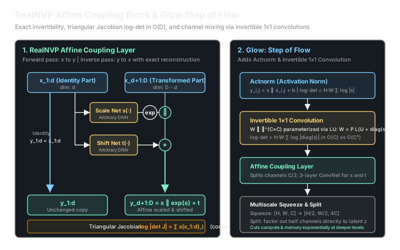
RealNVP circumvents this with affine coupling layers. The input vector $x \in \mathbb{R}^D$ is partitioned along feature dimensions into two parts: $x_{1:d}$ and $x_{d+1:D}$ , where $d < D$ . The forward transformation $y = f(x)$ is defined as:

y_{1:d} = x_{1:d}

y_{d+1:D} = x_{d+1:D} \odot \exp(s(x_{1:d})) + t(x_{1:d})

Here, $s: \mathbb{R}^d \to \mathbb{R}^{D-d}$ is a scale network and $t: \mathbb{R}^d \to \mathbb{R}^{D-d}$ is a translation network. Crucially, $s$ and $t$ can be arbitrarily complex neural networks (such as deep residual convolutional networks) with no invertibility constraints of their own.

Because $y_{1:d}$ depends only on $x_{1:d}$ , and $y_{d+1:D}$ depends on $x_{1:d}$ and $x_{d+1:D}$ , the Jacobian matrix is lower triangular:

J = \frac{\partial y}{\partial x} = \begin{bmatrix} I_d & 0 \\ \frac{\partial y_{d+1:D}}{\partial x_{1:d}} & \operatorname{diag}(\exp(s(x_{1:d}))) \end{bmatrix}

The determinant of a triangular matrix is the product of its diagonal elements. Its log-determinant reduces to a simple sum that evaluates in $\mathcal{O}(D)$ linear time:

\log |\det J| = \sum_{i=1}^{D-d} s(x_{1:d})_i

The exact inverse requires no matrix inversion:

x_{1:d} = y_{1:d}

x_{d+1:D} = (y_{d+1:D} - t(y_{1:d})) \odot \exp(-s(y_{1:d}))

Glow enhances RealNVP by organizing transformations into a repeating Step of Flow containing three components:

Actnorm (Activation Normalization): Replaces batch normalization with an affine transformation $y_{i,j} = s \odot x_{i,j} + b$ with per-channel scale $s$ and bias $b$ initialized to give zero mean and unit variance on the first batch. The log-determinant is $h \cdot w \cdot \sum \log |s|$ .
Invertible $1 \times 1$ Convolution: Generalizes channel permutation. For a tensor of shape $h \times w \times c$ , a weight matrix $W \in \mathbb{R}^{c \times c}$ mixes channels: $y = x W$ . Parameterizing $W$ via LU decomposition ( $W = P L (U + \operatorname{diag}(s))$ ) allows evaluating $\log |\det W| = h \cdot w \cdot \sum \log |s|$ in $\mathcal{O}(c)$ time.
Affine Coupling Layer: Applies the RealNVP split-scale-shift mechanism.

Worked Example

Let us trace a single affine coupling block on a 4-dimensional vector $x = [2.0, -1.0, 3.0, 4.0]$ where $D=4$ and $d=2$ .

Split input into two halves: $x_{1:2} = [2.0, -1.0], \quad x_{3:4} = [3.0, 4.0]$
Evaluate arbitrary neural networks $s(x_{1:2})$ and $t(x_{1:2})$ . Suppose the network outputs: $s(x_{1:2}) = [0.4, 0.1], \quad t(x_{1:2}) = [0.0, -0.3]$
Compute scaling factors via exponentiation: $\exp(s) = [\exp(0.4), \exp(0.1)] = [1.49182, 1.10517]$
Compute output $y$ : $y_{1:2} = x_{1:2} = [2.0, -1.0]$ $y_3 = 3.0 \times 1.49182 + 0.0 = 4.47546$ $y_4 = 4.0 \times 1.10517 + (-0.3) = 4.42068 - 0.3 = 4.12068$ $y = [2.0, -1.0, 4.47546, 4.12068]$
Compute the contribution to log-likelihood (the Jacobian log-determinant): $\log |\det J| = s_1 + s_2 = 0.4 + 0.1 = 0.5000$
Invert from $y = [2.0, -1.0, 4.47546, 4.12068]$ back to $x$ : $x_{1:2} = y_{1:2} = [2.0, -1.0]$ $s(y_{1:2}) = [0.4, 0.1], \quad t(y_{1:2}) = [0.0, -0.3]$ $x_3 = (4.47546 - 0.0) \times \exp(-0.4) = 4.47546 \times 0.67032 = 3.0000$ $x_4 = (4.12068 - (-0.3)) \times \exp(-0.1) = 4.42068 \times 0.90484 = 4.0000$ The reconstruction is numerically exact.

Code

1from typing import Tuple2import math3
4class AffineCouplingLayer:5    """Affine coupling layer operating on vectors with exact inversion."""6
7    def __init__(self, dim: int) -> None:8        self.dim = dim9        self.split_dim = dim // 210        # Weights for simple linear mappings modeling s and t11        self.w_s = [0.2, -0.1]12        self.w_t = [-0.5, 0.3]13        self.b_t = [1.0, 0.0]14
15    def _net(self, x1: list[float]) -> Tuple[list[float], list[float]]:16        # Scale s and translation t conditioned on x117        s = [self.w_s[0] * x1[0], self.w_s[1] * x1[1]]18        t = [self.w_t[0] * x1[0] + self.b_t[0], self.w_t[1] * x1[1] + self.b_t[1]]19        return s, t20
21    def forward(self, x: list[float]) -> Tuple[list[float], float]:22        x1 = x[:self.split_dim]23        x2 = x[self.split_dim:]24        s, t = self._net(x1)25
26        y1 = list(x1)27        y2 = [x2[i] * math.exp(s[i]) + t[i] for i in range(len(x2))]28        log_det = sum(s)29        return y1 + y2, log_det30
31    def inverse(self, y: list[float]) -> list[float]:32        y1 = y[:self.split_dim]33        y2 = y[self.split_dim:]34        s, t = self._net(y1)35
36        x1 = list(y1)37        x2 = [(y2[i] - t[i]) * math.exp(-s[i]) for i in range(len(y2))]38        return x1 + x239
40
41layer = AffineCouplingLayer(dim=4)42x_in = [2.0, -1.0, 3.0, 4.0]43y_out, log_det_val = layer.forward(x_in)44x_recovered = layer.inverse(y_out)45
46print("Forward y:", [round(v, 4) for v in y_out])47# -> Forward y: [2.0, -1.0, 4.4755, 4.1207]48print("Log det:", round(log_det_val, 4))49# -> Log det: 0.550print("Reconstructed x:", [round(v, 4) for v in x_recovered])51# -> Reconstructed x: [2.0, -1.0, 3.0, 4.0]

Watch Out For

Numerical explosion from unconstrained exponential scaling

Symptom: During training, loss becomes NaN or sudden gradient explosions occur within the coupling layers after a few thousand steps.

In an affine coupling layer, $y_2 = x_2 \odot \exp(s(x_1)) + t(x_1)$ . If the neural network $s(x_1)$ outputs unbounded activations like $s_i = 15.0$ , $\exp(s_i) \approx 3.26 \times 10^6$ . The inverse operation multiplies by $\exp(-s_i)$ , resulting in severe numerical underflow and vanishing gradients.

The remedy is to pass the scale network outputs through a bounding activation: $s = \alpha \cdot \tanh(\tilde{s})$ where $\alpha \approx 2.0$ , or clamp $\exp(s)$ to $[\epsilon, 1/\epsilon]$ . This guarantees stable conditioning throughout both forward and reverse paths.

The Quick Version

Normalizing flows chain bijective layers to map complex empirical data distributions into simple isotropic Gaussians.
RealNVP splits feature dimensions in half, applying identity to the first half and affine scale-and-shift to the second half.
Triangular Jacobians reduce determinant computation from an intractable $\mathcal{O}(D^3)$ to linear $\mathcal{O}(D)$ time.
Glow extends RealNVP with actnorm and invertible $1 \times 1$ convolutions to mix channels without fixed permutations.
Both exact log-likelihood evaluation and sample synthesis execute in a single parallelizable forward pass.