Bayesian Decision Theory

The best prediction is not always the best decision. Bayesian decision theory weighs each action by posterior chance times real-world cost.

A 0.3 spam posterior with a 10-to-1 miss cost makes flagging cheaper at 0.7 than keeping at 3.0

Why Does This Exist?

Classifiers output probabilities; products take actions. Missing spam costs a click, missing fraud costs thousands, and the two demand different thresholds on the same posterior. Accuracy-maximizing rules ignore the asymmetry and bleed money.

Decision theory closes the gap: pick $a$ minimizing posterior expected loss $\\rho(a \\mid x) = \\int L(\\theta, a)\\,p(\\theta \\mid x)\\,d\\theta$ . Squared loss gives the posterior mean, absolute loss the median, 0-1 loss the MAP. It builds on Bayesian inference and corrects the point estimates in MAP estimation.

The one idea you need first

A loss $L(\\theta, a)$ prices being wrong: 0 for right, positive for wrong, asymmetric when misses hurt more. The posterior $p(\\theta \\mid x)$ says where $\\theta$ likely sits. Multiply and integrate.

Think of It Like This

Umbrellas and ruined suits

Rain chance is 30%. An umbrella costs carrying it; a ruined suit costs ten times more. The MAP forecast says no rain, but the loss-aware commuter carries the umbrella because $0.3 \\times 10 > 0.7 \\times 1$ .

Same forecast, different action, because costs differ. Where it stops: weather losses are personal and stable, while business losses shift with context and must be re-estimated per decision.

How It Actually Works

Steps: infer posterior, price actions with $L$ , minimize $\\rho$ . Closed forms: squared error $\\to$ mean $\\mathbb{E}[\\theta \\mid x]$ ; absolute $\\to$ median; 0-1 $\\to$ mode (MAP); asymmetric linear $\\to$ posterior quantile. Frequentist risk $R(\\theta, \\delta) = \\mathbb{E}_X[L(\\theta, \\delta(X))]$ averages over data instead; Bayes risk averages over the prior too.

Worked example

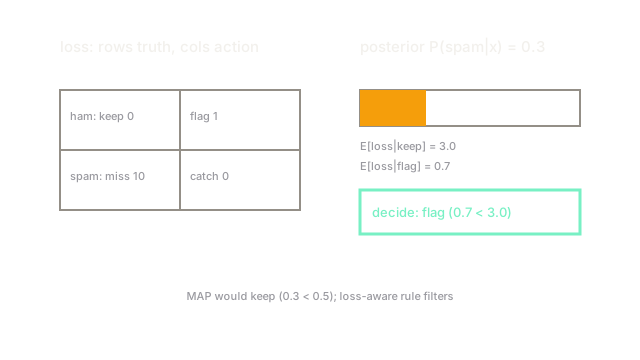
Spam filter, $P(\\text{spam} \\mid x) = 0.3$ . Losses: miss $= 10$ , false flag $= 1$ , correct $= 0$ . Expected loss of keep: $0.3 \\times 10 + 0.7 \\times 0 = 3.0$ . Of flag: $0.3 \\times 0 + 0.7 \\times 1 = 0.7$ . Flag wins $0.7 < 3.0$ though ham is likelier. Threshold form: flag when $P(\\text{spam}) > 1/11 \\approx 0.0909$ . At 0.3 the rule fires confidently.

Code

1p_spam, miss, false_flag = 0.3, 10.0, 1.02keep = p_spam * miss  # 3.03flag = (1 - p_spam) * false_flag  # 0.74print(round(keep, 2), round(flag, 2))  # -> (3.0, 0.7)5print("flag" if flag < keep else "keep")  # -> flag

Loss arithmetic overrides the 0.5 intuition. The threshold $1/11$ generalizes to any cost pair.

Watch Out For

Thresholding at 0.5 under asymmetric cost

Default 0.5 thresholds assume symmetric loss. With 10-to-1 costs the optimal cutoff sits near 0.09, so 0.5 lets most costly misses through. Fraud, medical, and safety teams pay for this default.

Set the threshold from $L$ , not habit: flag when $p > L_{FP}/(L_{FP} + L_{FN})$ . Recalibrate probabilities first.

Hiding the loss function from review

Undocumented costs make decisions unauditable: nobody can tell whether flagging was brave or the loss matrix was rigged. Stakeholders then relitigate every call.

Publish $L$ with the model card and version it. If costs change, re-derive the rule rather than nudging thresholds.

The Quick Version

Decide by minimizing posterior expected loss, not by maximizing posterior probability.
Squared loss gives the mean, absolute the median, 0-1 the MAP.
Spam at 0.3 with 10-to-1 costs filters because $0.7 < 3.0$ ; threshold near 0.09.
MAP is the special case of symmetric 0-1 loss, not the default decision.
Thresholds come from the loss ratio; calibrate probabilities before applying them.
Version the loss matrix with the model for auditable decisions.