Math

MAP Estimation

Maximum likelihood with an opinion added: multiply the likelihood by a prior before maximising, and the penalty terms you already use for regularisation fall out of the algebra.

MAP multiplies the likelihood by a prior and takes the peak of the product, so the estimate sits between where the data points and where the prior points — and moves toward the data as more of it arrives

Why Does This Exist?

Because weight decay is not a trick, and treating it as one costs you the ability to reason about it.

Every training script you have written contains a regularisation term. In PyTorch it is weight_decay=0.01 on the optimiser. In scikit-learn it is alpha on Ridge or C on a linear model. The standard explanation is "it stops overfitting by keeping the weights small", which is true and explains nothing: it does not say why squared weights rather than absolute ones, it does not say what value to pick, and it does not say what the value means.

MAP estimation says exactly what it is. An L2 penalty is a Gaussian prior on the weights. An L1 penalty is a Laplace prior. The coefficient is not a free knob — it is a ratio of two variances, one belonging to your noise model and one to your prior belief. Once you can read it that way, three things become answerable:

Why does the best regularisation strength shrink as the dataset grows? Because the coefficient is a fixed prior competing against a likelihood that grows with $n$ . The prior does not get weaker; the data gets louder.
Why does L1 produce exact zeros where L2 does not? Because the Laplace distribution has a spike at zero and the Gaussian does not. It is a property of the prior's shape, visible on a plot.
What does weight_decay=0.01 actually assert? That before seeing any data you believed each weight was drawn from a zero-mean Gaussian of a particular width. You can compute the width.

MAP is also the honest halfway house. Full Bayesian inference gives you a whole posterior distribution and costs an intractable integral. Maximum likelihood gives you a point and no way to express prior knowledge. MAP gives you a point and a place to put prior knowledge, for essentially no extra compute — which is why it, and not full Bayes, is what deep learning actually runs.

Think of It Like This

A new player's batting average after three innings

A cricketer joins your team and scores 0, 0 and 90 in their first three innings. Their average is 30.

What do you predict for the next innings? Not 30. You know something before the data arrived: professional batters mostly average between 20 and 50, a duck is common, and a 90 is a good day rather than a new baseline. Three innings is not enough to overturn that.

So you land somewhere between what the data says and what you knew — and importantly, closer to what you knew, because you know a lot and the data is thin.

Now the season progresses. After forty innings they average 30. Now you predict 30. Your prior has not changed and has not weakened; it has simply been outvoted. Forty innings is real evidence and the prior was never claiming certainty.

That is the whole mechanism, and three features of it transfer exactly:

The prior is a distribution, not a guess. "Batters average 20 to 50" is a shape with a centre and a width. A narrow prior resists the data hard; a wide one barely resists at all. This width is the regularisation strength.

The data wins eventually, and at a known rate. The likelihood's influence grows with sample size while the prior's stays fixed. MAP converges on the maximum likelihood estimate as $n \to \infty$ .

You get one number, not a range. The analogy naturally produces a range — "probably 25 to 35" — and MAP throws that away, keeping only the single most likely value. That is the sacrifice, and the second pitfall is what it costs.

How It Actually Works

Bayes' theorem with $\theta$ for the parameters and $D$ for the data:

p(\theta \mid D) = \frac{p(D \mid \theta)\, p(\theta)}{p(D)}

MAP takes the $\theta$ that maximises the left-hand side. The denominator $p(D)$ does not depend on $\theta$ , so it can be dropped — and this is the whole reason MAP is cheap, because that denominator is the intractable integral described in integrals in probability:

\hat{\theta}_{\mathrm{MAP}} = \arg\max_{\theta}\ p(D \mid \theta)\, p(\theta)

In plain words: pick the parameters that make the data likely and are themselves plausible. Take logs, since products of many small numbers underflow and sums are what optimisers want:

\hat{\theta}_{\mathrm{MAP}} = \arg\max_{\theta}\ \big[\log p(D \mid \theta) + \log p(\theta)\big]

Negate to get something to minimise, and the shape of every loss function you have written appears:

\hat{\theta}_{\mathrm{MAP}} = \arg\min_{\theta}\ \big[\underbrace{-\log p(D \mid \theta)}_{\text{your loss}} + \underbrace{-\log p(\theta)}_{\text{your penalty}}\big]

The regularisation term is the negative log prior. Not analogous to it. It is it. Drop the prior — assume every parameter value equally plausible — and the second term is a constant, MAP collapses to maximum likelihood, and you are training unregularised.

A Gaussian prior gives you L2, with the coefficient derived

Take linear regression. The likelihood is Gaussian noise of variance $\sigma^2$ around the model's predictions, so the negative log-likelihood is the familiar sum of squares:

-\log p(D \mid w) = \frac{1}{2\sigma^2}\lVert y - Xw \rVert_2^2 + \text{const}

Now put a zero-mean Gaussian prior of variance $\tau^2$ on each weight, independently:

-\log p(w) = \frac{1}{2\tau^2}\lVert w \rVert_2^2 + \text{const}

Add them and multiply through by $2\sigma^2$ , which changes nothing about where the minimum sits:

\hat{w}_{\mathrm{MAP}} = \arg\min_{w}\ \lVert y - Xw \rVert_2^2 + \lambda \lVert w \rVert_2^2, \qquad \lambda = \frac{\sigma^2}{\tau^2}

That is ridge regression, and the penalty coefficient has a meaning: $\lambda$ is the noise variance divided by the prior variance. Everything follows from reading it.

Narrow prior, small $\tau^2$ : strong belief the weights are near zero, large $\lambda$ , heavy shrinkage.
Wide prior, large $\tau^2$ : no real belief, $\lambda \to 0$ , back to plain least squares.
Noisy data, large $\sigma^2$ : the likelihood is less trustworthy, so $\lambda$ rises and the prior takes over. Regularise more when your labels are noisy, and this says why.

The closed form is $\hat{w} = (X^\top X + \lambda I)^{-1} X^\top y$ — the least squares normal equations with $\lambda$ added down the diagonal. That addition makes the matrix strictly positive definite and therefore invertible even when $X^\top X$ is singular, which is the numerical reason ridge works on collinear or wide data where ordinary least squares has no unique solution at all.

A Laplace prior gives you L1

Swap in a Laplace (double-exponential) prior, $p(w_j) \propto \exp(-\lvert w_j \rvert / b)$ :

-\log p(w) = \frac{1}{b} \lVert w \rVert_1 + \text{const}

and you have lasso. The reason it produces exact zeros is visible in the prior's shape rather than in any optimisation detail. A Gaussian is flat at zero — its derivative there is zero — so there is no pressure to sit exactly at zero rather than nearby. The Laplace has a kink: its derivative is $\pm 1/b$ right up to the origin, so a constant force pushes each weight toward zero until the data pushes back hard enough. Weights the data does not care about get pinned exactly at zero.

The pattern generalises. Pick a prior, take its negative log, and you have designed a penalty. This is where group lasso, elastic net and spike-and-slab priors come from, and it is a better way to invent a regulariser than guessing at an algebraic form.

Worked example

The cleanest case to check by hand is a coin, because both the likelihood and the prior have simple closed forms.

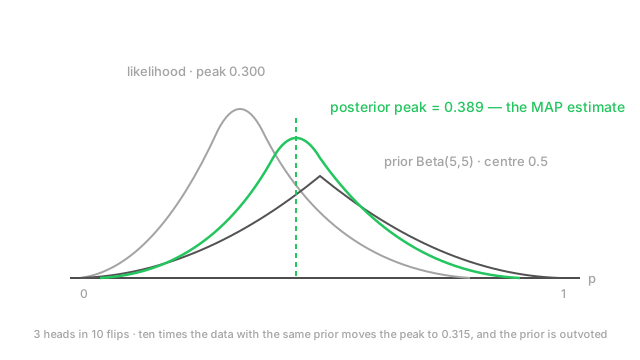
Ten flips, three heads. The maximum likelihood estimate is the obvious one:

\hat{p}_{\mathrm{MLE}} = \frac{3}{10} = 0.300

Now add a Beta prior. A $\mathrm{Beta}(\alpha, \beta)$ prior on a coin's bias behaves exactly like having already seen $\alpha - 1$ heads and $\beta - 1$ tails before the experiment started — the cleanest intuition for a prior anywhere in statistics. The MAP estimate is then the same fraction with those pseudo-counts folded in:

\hat{p}_{\mathrm{MAP}} = \frac{h + \alpha - 1}{n + \alpha + \beta - 2}

With $\mathrm{Beta}(2,2)$ — a gentle nudge toward fairness, worth one pseudo-head and one pseudo-tail:

\hat{p}_{\mathrm{MAP}} = \frac{3 + 1}{10 + 2} = \frac{4}{12} = 0.333

With $\mathrm{Beta}(5,5)$ — a firmer belief, worth four of each:

\hat{p}_{\mathrm{MAP}} = \frac{3 + 4}{10 + 8} = \frac{7}{18} = 0.389

In plain words: 0.300, 0.333, 0.389 — the same three heads in ten, pulled toward 0.5 by an amount set entirely by how firm the prior is.

Now hold the prior fixed at $\mathrm{Beta}(5,5)$ and multiply the data by ten. A hundred flips, thirty heads, same 30% rate:

\hat{p}_{\mathrm{MAP}} = \frac{30 + 4}{100 + 8} = \frac{34}{108} = 0.315

The estimate has moved from 0.389 back to 0.315, closing most of the gap to the MLE's 0.300. The prior is identical. It has simply been outvoted, and eight pseudo-observations against a hundred real ones is not a fair fight. This is what "the data wins eventually" looks like arithmetically, and it is the same reason weight_decay needs retuning when your dataset grows by an order of magnitude.

One more reading of the same numbers. The Beta(5,5) prior is worth 8 pseudo-observations, so at $n = 8$ the prior and the data have equal say. That number is the useful way to express any regularisation strength: not " $\lambda = 0.01$ " but "the prior is worth about this many examples".

Show Me the Code

1import numpy as np2
3
4def map_coin(heads: int, n: int, alpha: float, beta: float) -> float:5    """Posterior mode of a Beta-Binomial: alpha-1 and beta-1 act as pseudo-counts."""6    return (heads + alpha - 1) / (n + alpha + beta - 2)7
8
9print(round(map_coin(3, 10, 1, 1), 3))    # -> 0.3     flat prior == MLE10print(round(map_coin(3, 10, 2, 2), 3))    # -> 0.333   gentle pull toward 0.511print(round(map_coin(3, 10, 5, 5), 3))    # -> 0.389   firmer pull12print(round(map_coin(30, 100, 5, 5), 3))  # -> 0.315   same prior, 10x the data13
14# Ridge IS a Gaussian prior: lambda = noise variance / prior variance.15X = np.array([[1.0, 1.0], [1.0, 2.0], [1.0, 3.0]])   # (3, 2): intercept column, then x16y = np.array([1.0, 2.0, 3.3])                        # (3,)17penalty = np.diag([0.0, 1.0])                        # the 0.0 spares the intercept18for lam in (0.0, 1.0, 100.0):19    w = np.linalg.solve(X.T @ X + lam * penalty, X.T @ y)20    print(lam, np.round(w, 3))   # slope 1.15 -> 0.767 -> 0.023 as the prior tightens21
22bad = np.linalg.solve(X.T @ X + 100 * np.eye(2), X.T @ y)23print(np.round(bad, 3))          # -> [0.054 0.128]: the slope went UP, not down

The first four lines reproduce the worked example exactly. The loop shows the same mechanism in the linear case: at $\lambda = 0$ the slope fits the data, at $\lambda = 100$ the prior has flattened it to almost nothing and the intercept has absorbed the mean. Adding $\lambda$ to the diagonal is the only difference between these and the ordinary normal equations.

The last line is the first pitfall in one number. Swapping the mask for np.eye(2) penalises the intercept too, and the intercept collapses from 2.055 to 0.054 — but the slope rises from 0.023 to 0.128, a factor of 5.7, because it is now the only thing left that can reach the data. Tightening an L2 penalty made a coefficient larger. That is the signature of a prior applied to a term the prior was never about.

Watch Out For

Regularising the intercept, or regularising unscaled features

Two versions of one mistake: applying a prior to something the prior was never about.

The intercept. A zero-mean prior on a weight says "this feature probably does not matter much". Applied to the bias term it says "the target is probably near zero", which is a claim about your units, not your model. Shift your labels from Celsius to Kelvin and a penalised intercept changes your predictions. The code above shows the consequence directly: penalising the intercept crushes it from 2.055 to 0.054 and inflates the slope from 0.023 to 0.128, so strengthening the penalty made a coefficient bigger. The correct treatment is to leave the intercept out of the penalty — scikit-learn's Ridge does this for you, and a naive X.T @ X + lam * np.eye(d) does not. In PyTorch, weight_decay on a bare optim.AdamW(model.parameters()) hits every bias and every LayerNorm gain. The standard fix is two parameter groups, one with decay and one without, and it is a measurable difference on small models rather than a purity concern.

Unscaled features. An L2 penalty is $\sum_j w_j^2$ , which treats every weight identically. But a feature measured in millimetres needs a weight a thousand times larger than the same feature in metres to have the same effect, and squaring makes that a million-fold difference in penalty. The prior you meant to be uniform across features is now determined by your units. A feature in the millions — a salary, a population count — gets its coefficient crushed to nothing while a feature in the range 0 to 1 goes almost unpenalised.

The rule: standardise before you regularise, and keep the scaler inside your cross-validation pipeline so the fold statistics are not leaking. If a feature genuinely deserves a different prior, set it deliberately with a per-feature penalty rather than through an accident of measurement.

Treating the MAP estimate as if it summarised the posterior

MAP returns the posterior's highest point. That is a weaker claim than it sounds, and in high dimensions it is nearly vacuous.

The mode is not the mean, and for a skewed posterior it is not representative. For the $\mathrm{Beta}(5,9)$ posterior in the worked example the mode is $0.333$ and the mean is $5/14 = 0.357$ . A small gap here, but it grows with skew, and for variance or scale parameters the mode can sit far from any typical value.

In high dimensions the mode has almost no probability mass near it. This is the concentration-of-measure result and it is genuinely counterintuitive: for a 1,000-dimensional Gaussian, samples land at a radius of about $\sqrt{1000} \approx 31.6$ standard deviations from the mean, in a thin shell. The mode is the single most likely point, and simultaneously a place the distribution essentially never visits. Optimising to it is fine; describing the posterior by it is not.

The mode is not invariant under reparameterisation, and the mean is. Estimate a variance by MAP, then estimate the log-variance by MAP, then exponentiate: you get two different answers from the same data and the same prior. This is the change of variables Jacobian at work — the density gets rescaled by the transform, so its peak moves. A posterior mean does not have this problem. If someone asks whether you parameterised by $\sigma$ , $\sigma^2$ or $\log \sigma$ , this is why the question matters.

The consequence for practice is the honest one: a MAP-trained network's softmax output is not a calibrated probability. It is a point estimate that ignores parameter uncertainty entirely, which is a large part of why deep networks are confidently wrong on out-of-distribution inputs. If you need uncertainty, you need something that keeps more of the posterior than its peak — a Laplace approximation around the MAP, deep ensembles, or MC dropout, all covered from Bayesian inference. Temperature scaling patches the symptom on in-distribution data and does not touch the cause.

The Quick Version

MAP maximises the posterior instead of the likelihood: $\arg\max_\theta\ p(D \mid \theta)\, p(\theta)$ .
The Bayes denominator drops out because it does not depend on $\theta$ . That is why MAP is cheap and full Bayes is not.
In negative-log form the objective is loss plus penalty, and the penalty is the negative log prior. Regularisation is not analogous to a prior; it is one.
A Gaussian prior gives L2 (ridge) with $\lambda = \sigma^2 / \tau^2$ — noise variance over prior variance. A Laplace prior gives L1 (lasso).
L1 zeroes weights because the Laplace prior has a kink at the origin and the Gaussian is flat there.
Adding $\lambda I$ makes $X^\top X$ invertible, so ridge has a unique solution where ordinary least squares does not.
MAP converges to MLE as the data grows. Express the strength as "worth this many examples" to see why it needs retuning at a new dataset size.
Never penalise the intercept, and standardise features first, or your units are choosing your prior.
MAP gives a point, not a posterior. In high dimensions the mode is not where the mass is, and it is not invariant under reparameterisation.