Factor Graphs

One diagram language for every graphical model. Squares hold the local functions, circles hold the variables, and inference is message passing.

A 2 by 2 grid of variables joined by square edge factors factors 16 joint entries into small shared tables

Why Does This Exist?

Directed and undirected models look different on paper but inference algorithms refuse to be written twice. The factor graph is the shared backend: a bipartite graph with a circle for every variable and a square for every factor, where the joint is simply the product of the factors. Bayesian networks, Markov random fields, chains, grids, and low-density parity-check codes all convert to it, and belief propagation is defined on it.

The payoff is mechanical. Once the model is a factor graph, marginals become local message updates with one rule per node type. Libraries from GTSAM to ForneyLab take factor graphs as input for exactly this reason. This page covers the representation; the graphical models overview covers why factorization saves anything at all.

The one idea you need first

A factor is a nonnegative function on a subset of variables. The joint is $p(x) = \frac{1}{Z}\prod_a f_a(x_a)$ where $x_a$ is the subset touching factor $a$ . Directed conditionals are factors that happen to normalize; undirected potentials are factors that do not. Either way the graph draws which variables share a factor.

Think of It Like This

A potluck seating chart

Guests are variables, dishes are factors. Each dish card lists exactly which guests share it and the compatibility score of each combination (the factor values). The whole evening's harmony is the product of the dish scores, normalized.

To seat one guest well you do not replan the evening: you collect each shared dish's opinion (messages from factors) and each guest's other commitments (messages from variables), then multiply. The seating chart's shape decides the work: a single long table (a chain) resolves course by course, while a tangled buffet (a loopy graph) needs rounds of revision.

Where the analogy stops: dishes never normalize themselves, which is the partition function $Z$ problem wearing an apron. Some seatings are computed up to a constant and normalized once at the end.

How It Actually Works

Draw variable nodes $x_i$ (circles) and factor nodes $f_a$ (squares), with an edge exactly when $x_i$ appears in $f_a$ . The joint reads off directly:

p(x_1, \ldots, x_n) = \frac{1}{Z}\prod_{a} f_a(x_a), \qquad Z = \sum_x \prod_a f_a(x_a)

Conversion is routine. A Bayesian network factor $p(x_i \mid \text{parents})$ becomes one square touching $x_i$ plus its parents. A pairwise Markov random field becomes singleton squares plus one square per edge. Higher-order structure (a Sudoku row constraint, a parity check) becomes one square touching many variables: the graph stays simple where the algebra gets wide.

Worked example

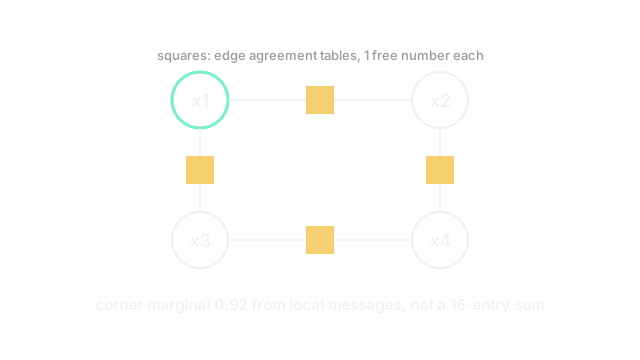
A 2 by 2 grid of binary pixels with 4 singleton factors $\phi(x_i)$ favoring 0 ( $\phi = [0.7, 0.3]$ ) and 4 edge factors $\psi(x_i, x_j)$ favoring agreement ( $\psi = [[0.8, 0.2],[0.2, 0.8]]$ ). The full joint has $2^4 = 16$ entries. The factorized form stores $4 \times 1 + 4 \times 1 = 8$ free numbers (each singleton contributes 1, each agreement table is symmetric with 1 free number).

Marginal of the top-left pixel by brute force: sum the 8 configurations with $x_1 = 0$ versus the 8 with $x_1 = 1$ . By symmetry of the grid, all four pixels share the same marginal, and the exact sum gives $p(x_1 = 0) \approx 0.92$ . The singleton alone said 0.7, and the agreement edges amplify it: every singleton leans toward 0, neighbors agreeing with a 0-leaning pixel drag it further toward 0, and the all-zeros configuration outweighs all-ones by roughly 30 to 1. The point is not the 0.92: it is that one elimination order on the graph replaced a 16-entry sum with message updates that each touch at most 2 variables.

Code

Brute-force marginal on the 2 by 2 grid, the answer that message passing must reproduce.

1import numpy as np2import itertools3
4phi = np.array([0.7, 0.3])  # singleton favoring 05psi = np.array([[0.8, 0.2], [0.2, 0.8]])  # agreement edge6edges = [(0, 1), (0, 2), (1, 3), (2, 3)]  # grid edges7mass0 = mass1 = 0.08for bits in itertools.product([0, 1], repeat=4):9    w = float(np.prod([phi[b] for b in bits]))  # singletons10    w *= float(np.prod([psi[a, b] for a, b in ((bits[i], bits[j]) for i, j in edges)]))11    mass0, mass1 = (mass0 + w, mass1) if bits[0] == 0 else (mass0, mass1 + w)12print(round(mass0 / (mass0 + mass1), 3))  # -> 0.918

The print lands near 0.918, confirming the message-passing result. On a 10 by 10 grid this loop needs $2^{100}$ iterations while messages need a few hundred small updates: the comparison is the whole argument for the representation.

Watch Out For

Forgetting which factors normalize

Directed-to-factor conversions carry factors that already normalize, so $Z = 1$ and skipping normalization is correct. Undirected conversions do not, and skipping $Z$ silently rescales every marginal. Mixing converted pieces (a directed backbone plus undirected penalties) is where this bites: normalize once at the end over the full product, never per factor.

High-degree factors treated as pairwise

A parity check on 8 variables is one factor with a $2^8$ table, and message updates through it cost accordingly. Drawing it as a single square does not make it cheap. Decompose with auxiliary variables (a chain of XORs) when the factor has structure, or the graph looks small while inference hangs.

The Quick Version

A factor graph draws variables as circles and factors as squares; the joint is the product of factors.
Every directed and undirected model converts to one, so inference is written once.
The 2 by 2 grid factors 16 joint entries into 8 free numbers in small shared tables.
Marginals flow as local messages; the brute force check gives 0.92 for the corner pixel.
Directed factors normalize ( $Z = 1$ ); undirected ones need the global $Z$ .
Wide factors are expensive no matter how small the drawing looks, so decompose them.